A casino claims a game is fair. A medical company says its test is accurate most of the time. A coach says a player makes free throws with probability \(0.8\). How can you tell whether the data are actually consistent with those claims? This question is at the heart of statistical inference: using observed results to decide whether a stated model for a random process is believable.
When a process is random, we should expect variation. Even if a coin is perfectly fair, it will not land heads exactly half the time in every short run. Even if a basketball player really makes \(80\%\) of free throws, that player can still miss several in a row. The challenge is to decide when a result is just ordinary randomness and when it is unusual enough to make us question the model.
Probability model is a mathematical description of a random process, including the possible outcomes and how likely each outcome is.
Data-generating process is the actual process that produces the outcomes we observe.
Consistent with a model means the observed result is reasonably likely to occur if the model is true.
A model does not need to predict the exact result. Instead, it predicts a range of plausible results. If the observed data fall in that range, the model is considered consistent with the data. If the data are very unlikely under the model, then the model may be questionable.
One of the most important ideas in probability is that rare events still happen. If something has probability \(0.01\), that does not mean it cannot occur. It means that in the long run, it happens about \(1\) time in \(100\) trials on average.
Suppose a fair coin has probability \(0.5\) of landing heads and probability \(0.5\) of landing tails on each spin. A result like \(5\) tails in a row sounds dramatic, but probability does not care whether a pattern seems dramatic to us. It only cares how often that pattern would occur in repeated trials.
Sequences that look "mixed" often feel more random to people than sequences with long runs, but both kinds of sequences can occur naturally. Human intuition about randomness is often weaker than the mathematics.
This is why statistics relies on numerical evidence. Instead of saying, "That seems too strange," we ask, "How likely is that result if the model is true?" That question turns a vague feeling into a mathematical judgment.
To test a model, we begin with a claim about how outcomes are generated. For example, a coin model might say that each spin is independent and that the probability of heads is \(0.5\). A manufacturing model might say that each item has a defect probability of \(0.02\). A sports model might say that a player makes a shot with probability \(0.75\).
The word independent matters. If one outcome affects the next, then the model changes. For instance, if a spinner becomes loose and starts favoring one side, then repeated outcomes may no longer match the original assumptions.
Observed data are consistent with a model when they do not look unusually far from what the model predicts. This does not prove the model is true. It only means the data do not strongly contradict it. On the other hand, if the data would be very rare under the model, then we have reason to doubt the model.
Consistency is about plausibility, not certainty. Statistical reasoning rarely gives a yes-or-no proof. Instead, it asks whether the observed result is plausible under a stated random process. If it is plausible, we keep the model as a possible explanation. If it is not plausible, we question the model and look for a better one.
This way of thinking is used throughout science. A scientist proposes a model, collects data, and asks whether the data are compatible with what the model predicts. If not, the model may need revision.
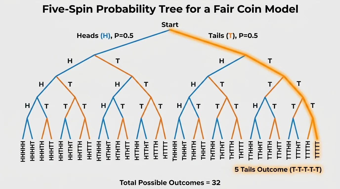
A classic example asks whether a model that says a spinning coin lands heads with probability \(0.5\) should be questioned after observing \(5\) tails in a row. A visual of all possible \(5\)-spin sequences helps explain why this outcome is rare but still completely possible under a fair-coin model.
As shown in [Figure 1], for \(5\) independent spins of a fair coin, each specific sequence has probability \(\left(\dfrac{1}{2}\right)^5 = \dfrac{1}{32}\). That includes the sequence \(\textrm{TTTTT}\), but it also includes \(\textrm{HTHTH}\), \(\textrm{HHTTT}\), and every other exact sequence of length \(5\).
There are \(2^5 = 32\) equally likely sequences in total. Only one of them is all tails, so the probability of getting \(5\) tails in a row is \(\dfrac{1}{32} = 0.03125\), or about \(3.125\%\).
Should that result make us question the model? The best answer is: maybe a little, but not strongly. A probability of about \(0.031\) is small, so the outcome is unusual. But it is not so incredibly rare that it would be shocking to see once in a while.
If the result had been \(10\) tails in a row, the probability under the fair-coin model would be \(\left(\dfrac{1}{2}\right)^{10} = \dfrac{1}{1024} \approx 0.00098\). That is less than \(0.1\%\), which gives much stronger reason to question the model.
The lesson is not that \(5\) tails proves the coin is unfair. It does not. Instead, it suggests we should compare the observed outcome with what the model says is typical or unusual. As we saw with the branching display in [Figure 1], even very neat-looking streaks are just one possible path in a random process.
Sometimes a probability can be calculated exactly, but sometimes simulation is easier and more realistic. A simulation uses technology or repeated random trials to imitate the model many times and see what kinds of results usually happen. The distribution of simulated outcomes makes it easier to compare an observed result with what the model predicts.
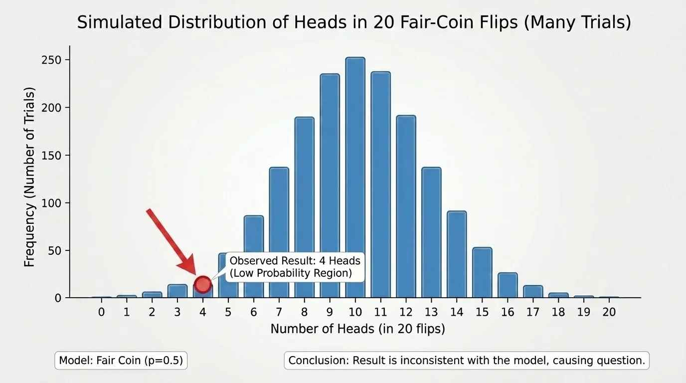
As shown in [Figure 2], suppose a model says a fair coin is flipped \(20\) times. You could simulate this process on a calculator or computer thousands of times. For each simulated trial, count how many heads appear. After many repetitions, you get a pattern of results: maybe most trials have around \(9\), \(10\), or \(11\) heads, while very few have only \(2\) heads or as many as \(18\).
This collection of repeated simulated results gives a picture of what is normal under the model. If your actual data fall near the center of that picture, the model seems reasonable. If your actual data fall far out in the tail, the model may be questionable.
Simulation is especially powerful because it turns an abstract claim into something you can inspect. Instead of asking only for one exact probability, you can ask how often outcomes at least as extreme as the observed result appear in the simulation.
For instance, if your observed result is only \(4\) heads in \(20\) flips, and only \(8\) out of \(1{,}000\) simulations produce \(4\) or fewer heads, then the estimated probability is \(\dfrac{8}{1000} = 0.008\). That would be strong evidence that the result is not very consistent with the fair-coin model.
From earlier probability work, recall that an estimated probability from simulation is found by dividing the number of times an event occurs by the total number of simulated trials. More simulations usually give a more stable estimate.
Simulation does not prove a model false, but it helps us judge how surprising the data are if the model were true. Later, formal statistical tests build on exactly this idea.
There is no universal line that separates "reasonable" from "unreasonable" in every situation, but statisticians often treat very small probabilities as evidence against a model. In many settings, results with probability below about \(0.05\) are considered unusual, and results below about \(0.01\) are considered very unusual.
These cutoffs are conventions, not laws of nature. Context matters. In medicine, where mistakes can be serious, stronger evidence may be required. In an informal classroom investigation, a rough judgment may be enough.
If the observed outcome has a small probability under the model, then one of two things may be true: either a rare event occurred, or the model is not a good description of the real process. Statistics helps us decide which explanation is more convincing.
"Random does not mean evenly spread; random means governed by probability."
This is why a surprising outcome does not automatically destroy a model. The right question is not "Could this happen?" but "How often should this happen if the model is correct?"
The following examples show how to judge consistency using either exact probability or simulation-based reasoning.
Worked example 1: Five tails in a row
A model says a spinning coin has probability \(0.5\) of heads and \(0.5\) of tails on each independent spin. You observe \(5\) tails in a row. Should you question the model?
Step 1: Find the probability of the observed sequence.
Because each tails result has probability \(\dfrac{1}{2}\), the probability of \(5\) tails in a row is \(\left(\dfrac{1}{2}\right)^5 = \dfrac{1}{32}\).
Step 2: Convert to a decimal or percent.
\(\dfrac{1}{32} = 0.03125\), which is about \(3.125\%\).
Step 3: Interpret the result.
This is unusual, but not impossible or extremely rare. It gives some reason to pay attention, but not strong enough reason by itself to reject the model.
The data are somewhat surprising but still reasonably possible under the model.
This first example shows the difference between a rare event and a nearly impossible one. That distinction is essential in statistical reasoning.
Worked example 2: Free throws
A player is modeled as making free throws with probability \(0.8\). In \(10\) shots, the player makes only \(4\). Is that consistent with the model?
Step 1: Identify what is being judged.
If the model is correct, then making only \(4\) out of \(10\) is a low result compared with the expected number \(10 \cdot 0.8 = 8\).
Step 2: Use simulation reasoning or exact probability reasoning.
If we simulate many sets of \(10\) shots with success probability \(0.8\), we would expect most results to be around \(7\), \(8\), or \(9\) makes. A result of \(4\) makes or fewer would appear only occasionally.
Step 3: Draw a conclusion.
A result this low is unusual, so it gives some evidence against the model. However, with only \(10\) shots, there is still substantial variability, so the evidence is not overwhelming.
The result is questionable but not conclusive. More shots would provide stronger evidence.
Short runs can be noisy. A player who truly shoots \(80\%\) can still have a bad stretch, especially in a small sample.
Worked example 3: Defective items
A factory model says \(2\%\) of items are defective. In a random sample of \(50\) items, you find \(5\) defective items. Should the model be questioned?
Step 1: Compare the observed result to the expected number.
The expected number of defective items is \(50 \cdot 0.02 = 1\).
Step 2: Judge how far the sample is from expectation.
Finding \(5\) defective items is much larger than the expected \(1\). A simulation of many samples of size \(50\) with defect probability \(0.02\) would likely show that \(5\) or more defects is fairly uncommon.
Step 3: Interpret in context.
Because the observed number is well above what the model predicts, there is meaningful evidence that the defect rate may be higher than \(0.02\), or that something in the process has changed.
This sample gives noticeable evidence against the model.
In manufacturing, this kind of reasoning matters because decisions about safety and quality often depend on whether observed defect counts fit the claimed process.
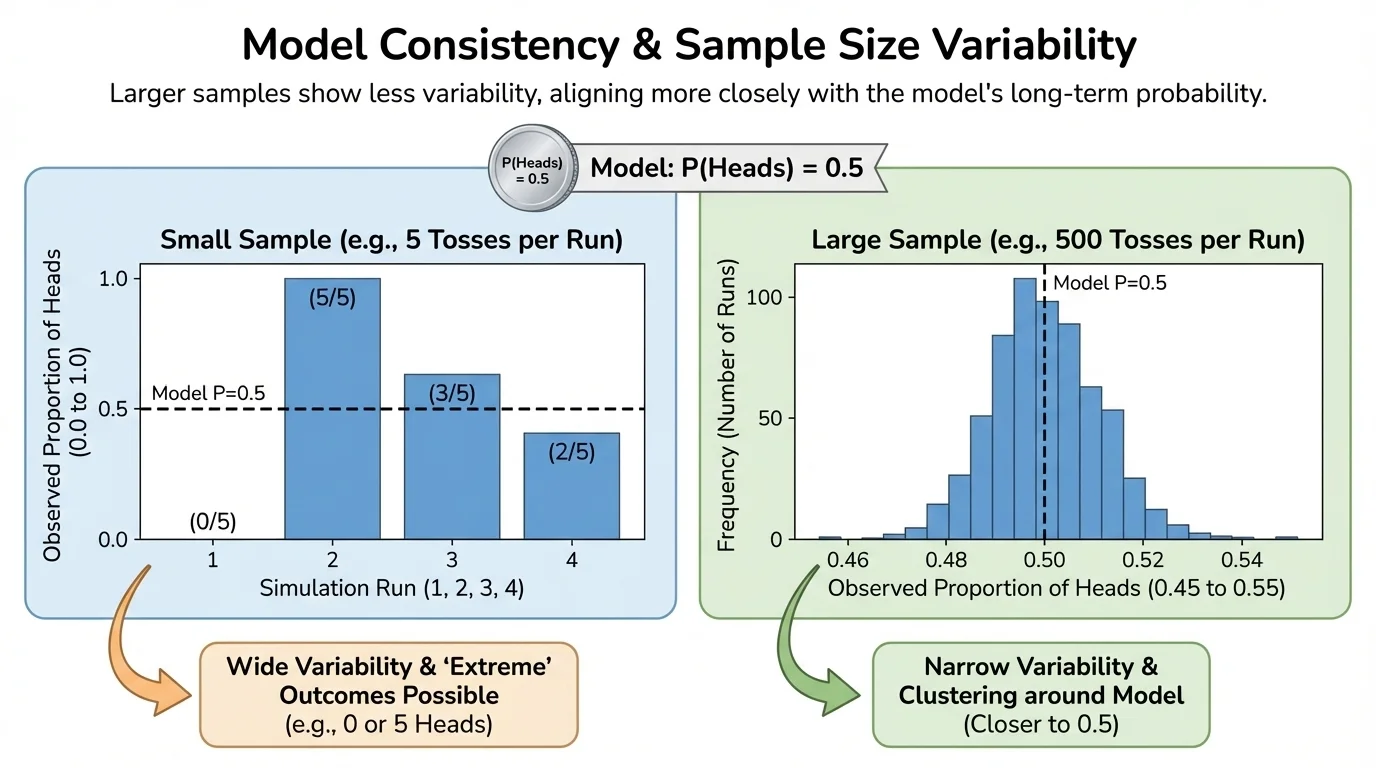
One of the most important ideas in the topic is that the same probability model can produce much more variable results in small samples than in large samples. This means sample size strongly affects how convincing the evidence is.
As illustrated in [Figure 3], suppose a coin is fair. In only \(4\) flips, getting \(3\) tails is not very surprising. In \(400\) flips, getting \(300\) tails would be astonishing. The larger the sample, the more stable the relative frequencies tend to be.
Small samples swing wildly. Large samples usually stay closer to the model's long-run probabilities. That is why one weird result in a tiny sample may mean little, while a strong pattern in a large sample can be powerful evidence.
Another important idea is that inconsistency with a model does not automatically identify the cause. If data do not fit the model, several explanations are possible: the probability may be wrong, the outcomes may not be independent, the sample may not be random, or there may be a measurement problem.
For example, if a survey result looks inconsistent with a model, that does not necessarily mean public opinion changed. It could mean the sample was biased. If coin spins look inconsistent with fairness, perhaps the spinner is damaged or perhaps the spins were not performed consistently.
This is why context matters. Statistics is not just calculation; it is reasoning about how the data were produced. The small-sample versus large-sample contrast in [Figure 3] reminds us that the strength of evidence depends heavily on how much data we have.
These ideas appear in many fields. In medicine, researchers ask whether the number of patients who improve under a treatment is consistent with what would happen by chance alone. In climate science, scientists compare observed data with models of natural variability. In sports analytics, teams ask whether a player's recent streak reflects true improvement or just randomness.
Election polling also depends on this reasoning. A poll does not expect to match the entire population exactly. Instead, analysts ask whether the poll's result is consistent with normal sampling variation or whether it suggests a real shift in support.
Manufacturing companies use this thinking to monitor quality. If the number of defective products suddenly becomes too high to be explained by ordinary variation, managers investigate the process. Financial analysts do something similar when deciding whether a surprising run of outcomes looks like random fluctuation or evidence that the system has changed.
| Situation | Model claim | Observed data | Main question |
|---|---|---|---|
| Coin spins | \(P(\textrm{heads}) = 0.5\) | Long streak of tails | Is the streak too rare under fairness? |
| Basketball | \(P(\textrm{make}) = 0.8\) | Unusually many misses | Bad luck or wrong model? |
| Manufacturing | \(P(\textrm{defect}) = 0.02\) | High defect count | Normal variation or process problem? |
| Polling | Stable support level | Poll far from expectation | Sampling variation or real change? |
Table 1. Examples of how consistency with a probability model is checked in different real-world settings.
One common mistake is assuming that a rare outcome proves the model is false. It does not. Rare things happen. A better conclusion is that the result provides evidence against the model, with strength depending on how rare the result is and how much data were collected.
Another mistake is believing that short-run results must match long-run probabilities exactly. A fair coin does not owe you heads after several tails. Randomness has no memory if the trials are independent.
A third mistake is ignoring the design of the data collection. If the process for collecting data is flawed, then even a good probability calculation may not answer the right question. Models only work well when their assumptions reasonably match reality.
Good statistical judgment combines mathematics and context. You calculate or simulate how surprising the data are under a model, and then you interpret that surprise in light of sample size, assumptions, measurement quality, and the consequences of being wrong.
When you decide whether data are consistent with a model, you are doing more than computing a number. You are asking whether the claimed random process gives a believable explanation for what actually happened.