A company can make money on a product even if some individual sales lose money. A casino can profit even when some players win. An insurance company can charge a premium lower than a rare disaster would cost. What connects all of these situations is one powerful idea: over many repeated trials, probability creates an average. That average is called the expected value, and it helps turn uncertainty into a number we can analyze.
In everyday life, many important choices involve uncertainty. A business may choose between two advertising plans. A student may enter a scholarship drawing. A driver may decide whether buying roadside coverage is worth the cost. In each case, no one knows exactly what will happen once, but probability helps us describe what tends to happen on average in the long run.
Expected value is useful because it combines two things at the same time: the value of each possible outcome and the probability of getting that outcome. A small reward with a high probability may be more valuable than a large reward with a tiny probability. Likewise, a rare but expensive loss can matter a lot.
To work with expected value, you need two ideas from earlier probability work: probabilities must be between 0 and 1, and the probabilities of all possible outcomes in a distribution must add to 1.
When mathematicians say expected value, they do not mean a guaranteed result. They mean the mean of the probability distribution, or the average outcome you would expect over many repetitions.
A random variable is a variable whose value depends on the outcome of a random process. For example, if you roll a die and let X be the number rolled, then X is a random variable. If you play a game and record your net profit, that profit can also be a random variable.
A probability distribution lists each possible value of the random variable and the probability of that value. For a fair die, the values are 1, 2, 3, 4, 5, and 6, and each has probability \(\dfrac{1}{6}\).
Not all distributions are uniform. Some outcomes may be much more likely than others. For example, suppose a store tracks the number of items a customer buys in one visit. The probabilities might not be equal at all. Expected value handles both equal and unequal probabilities.
Random variable: a quantity whose value is determined by chance.
Probability distribution: a list or table showing every possible value of a random variable and the probability of each value.
Expected value: the weighted mean of a random variable, found by multiplying each outcome by its probability and adding the results.
Because expected value is the mean of a distribution, it plays a role similar to the average in data analysis. The difference is that instead of averaging observed data values, we average possible outcomes using their probabilities as weights.
The key idea, as shown in [Figure 1], is that expected value is not an ordinary average where every outcome counts equally. It is a weighted mean, which means more likely outcomes count more heavily than less likely ones.
If a discrete random variable \(X\) can take values \(x_1, x_2, x_3, \dots\) with probabilities \(P(x_1), P(x_2), P(x_3), \dots\), then the expected value is
\[E(X) = \sum x \cdot P(x)\]
This means: multiply each outcome by its probability, then add all those products. If some outcomes are negative, include the negative signs. Negative outcomes often represent losses or costs.
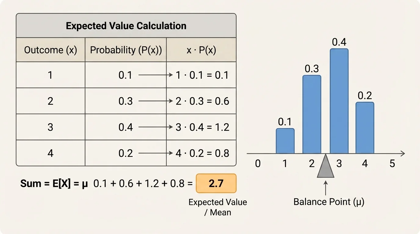
You can think of this as a balance point. If an outcome is large but unlikely, it pulls the average some amount. If an outcome is small but very likely, it may pull the average even more. That is why expected value can land between possible outcomes or even be a number that never occurs in a single trial.
Why the mean interpretation makes sense
If you repeat a random process many times and calculate the average of the actual results, that average tends to get closer to the expected value. In other words, expected value describes the long-run average outcome, not what must happen next.
For example, if the expected number of points from a game is \(2.7\), that does not mean you can score exactly \(2.7\) points in one play. It means that if the game were played many times, the average score per play would approach about \(2.7\).
To find expected value, use a clear process. First, identify every possible outcome. Second, identify the probability of each outcome. Third, multiply each outcome by its probability. Fourth, add the products.
If the random variable represents money won or lost, be sure to use the net outcome, not just the prize amount. For example, if a game costs $3 to play and you win $10, your net gain is $7, not $10. This detail is one of the most common sources of error.
| Outcome \(x\) | Probability \(P(x)\) | Product \(x \cdot P(x)\) |
|---|---|---|
| \(x_1\) | \(P(x_1)\) | \(x_1P(x_1)\) |
| \(x_2\) | \(P(x_2)\) | \(x_2P(x_2)\) |
| \(x_3\) | \(P(x_3)\) | \(x_3P(x_3)\) |
Table 1. General structure for calculating expected value from a discrete probability distribution.
Then compute
\[E(X) = x_1P(x_1) + x_2P(x_2) + x_3P(x_3) + \dots\]
Suppose a spinner has four equal sections labeled \(1\), \(2\), \(3\), and \(4\). Let \(X\) be the number the spinner lands on. Find \(E(X)\).
Worked example
Step 1: List the outcomes and probabilities.
The possible values are \(1, 2, 3, 4\). Since the spinner is fair, each probability is \(\dfrac{1}{4}\).
Step 2: Multiply each outcome by its probability.
\(1 \cdot \dfrac{1}{4} = \dfrac{1}{4}\), \(2 \cdot \dfrac{1}{4} = \dfrac{2}{4}\), \(3 \cdot \dfrac{1}{4} = \dfrac{3}{4}\), and \(4 \cdot \dfrac{1}{4} = \dfrac{4}{4}\).
Step 3: Add the products.
\(E(X) = \dfrac{1}{4} + \dfrac{2}{4} + \dfrac{3}{4} + \dfrac{4}{4} = \dfrac{10}{4} = 2.5\).
So the expected value is
\(E(X) = 2.5\)
This makes sense as the mean of the distribution. Even though the spinner never lands on \(2.5\), repeated spins would average close to \(2.5\).
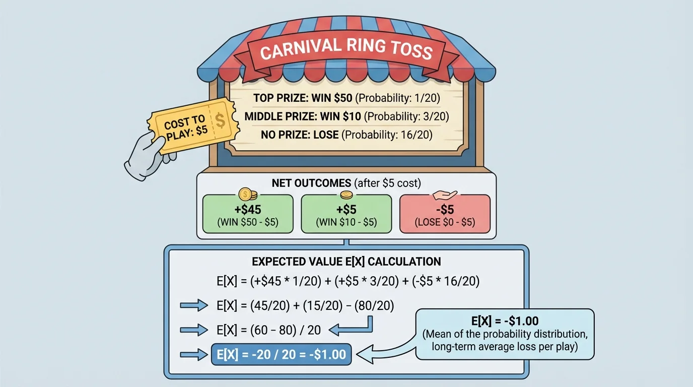
[Figure 2] shows why we must use net outcomes to analyze this game correctly. At a carnival, a game costs $2 to play. You have a probability of \(0.1\) of winning a $10 prize and a probability of \(0.9\) of winning nothing, so the possible net results are a gain of $8 or a loss of $2.
This question is really asking for the average profit per play. That makes expected value the right tool.
Worked example
Step 1: Identify the net outcomes.
If you win, your net gain is \(\$10 - \$2 = \$8\), so the outcome is \(+8\). If you do not win, you lose the $2 entry fee, so the outcome is \(-2\).
Step 2: Attach the probabilities.
\(P(+8) = 0.1\) and \(P(-2) = 0.9\).
Step 3: Compute the expected value.
\(E(X) = 8(0.1) + (-2)(0.9) = 0.8 - 1.8 = -1.0\).
The expected value is
\(E(X) = -1\)
This means that over many plays, the average result is a loss of $1 per play. A player might win on a single play, but in the long run the game favors the carnival. That is exactly why games like this can stay in business.
A teacher creates a multiple-choice bonus question. If a student answers correctly, they gain \(4\) points. If they answer incorrectly, they lose \(1\) point. If a student estimates a \(0.3\) chance of being correct, should they attempt the question?
Worked example
Step 1: Define the outcomes.
The random variable \(X\) is the change in score. The outcomes are \(+4\) and \(-1\).
Step 2: Use the probabilities.
\(P(+4) = 0.3\) and \(P(-1) = 0.7\).
Step 3: Calculate expected value.
\(E(X) = 4(0.3) + (-1)(0.7) = 1.2 - 0.7 = 0.5\).
The expected value is
\(E(X) = 0.5\)
Since the expected value is positive, the student gains an average of \(0.5\) points per attempt in the long run. Based on this estimate, attempting the question is a favorable choice.
Expected value is powerful, but it must be interpreted correctly. First, it describes a long-run average, not a guaranteed short-term result. A game with positive expected value can still lose money once. A medical treatment with a high expected benefit may still fail for one patient.
Second, expected value may not be a possible actual outcome. In Example 2, the expected value was \(-1\), but one play never results in exactly losing $1. You either gain $8 or lose $2. The expected value sits between actual outcomes because it represents the mean of the whole distribution.
Third, expected value is not the same as the most likely value. The probability of an outcome tells how likely that one outcome is. Expected value mixes all outcomes together into one average measure.
Insurance companies rely heavily on expected value. They know that one person may file a huge claim while many others file none, so they study long-run averages across very large groups.
That is why expected value is especially useful when a situation can be repeated many times, or when decisions affect many people or many transactions.
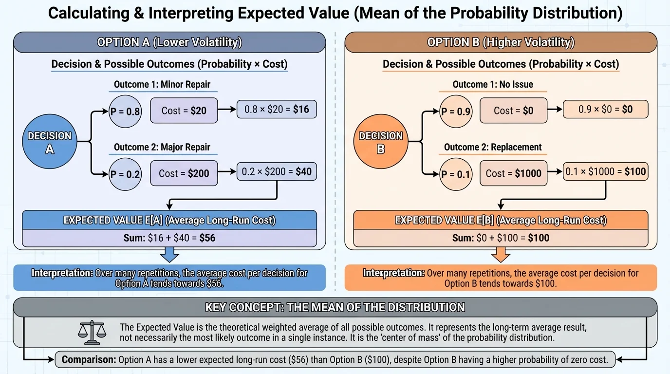
Expected value is often used to compare options. In a side-by-side decision, [Figure 3] illustrates how average long-run cost or profit can reveal which choice is better even when neither choice is certain.
Suppose a store offers an extended warranty for a laptop for $120. Without the warranty, there is a \(0.08\) chance of a repair costing $900 and a \(0.92\) chance of no repair cost. The expected repair cost without the warranty is \(900(0.08) + 0(0.92) = 72\), so the average long-run repair cost is $72. From a purely expected-value viewpoint, paying $120 for the warranty is not the better financial choice.
However, people do not always choose the option with the best expected value. Someone may prefer the warranty because they want to avoid the risk of a large one-time expense. Expected value helps evaluate the average outcome, but personal risk tolerance can still matter.
We can also compare business decisions. Suppose a company is deciding between two machines. Machine A has lower purchase cost but a higher chance of expensive repair. Machine B costs more at first but has a lower repair risk. Expected value allows the company to compare average long-run cost, not just sticker price. This same logic appears in finance, engineering, and economics.
Later, when you revisit these ideas in decision models, the side-by-side logic from [Figure 3] remains important: compare all possible outcomes, multiply by probabilities, and then compare averages.
One common mistake is forgetting to check that the probabilities add to \(1\). If they do not, the distribution is incomplete or incorrect.
Another common mistake is using gross prizes instead of net gains or losses. In the carnival example, the correct outcome when winning was \(+8\), not \(+10\), because the cost to play had to be included. [Figure 2] illustrates that distinction clearly.
A third mistake is confusing expected value with fairness. A game is often called fair if its expected value is \(0\) for the player. If \(E(X) > 0\), the player has an advantage. If \(E(X) < 0\), the game favors the house or the organizer.
Expected value also works when outcomes are decimals, negative numbers, or large amounts. For example, if a stock investment has possible one-year returns of \(-0.05\), \(0.04\), and \(0.12\) with certain probabilities, the same process applies. Multiply each return by its probability and add.
Expected value and fairness
If the expected gain from a game is zero, neither side has a long-run advantage. If the expected gain is negative for the player, then repeated play tends to produce losses for the player and gains for the organizer.
In advanced courses, expected value can also be used with continuous random variables, but at this level the main focus is on discrete distributions, where you can list all possible outcomes in a table.
Expected value appears in many serious fields. In medicine, researchers compare treatment options by looking at possible outcomes and their probabilities. In manufacturing, companies estimate average defect costs. In transportation, planners estimate delays and fuel use. In finance, investors compare average returns while also thinking about risk.
Sports analytics uses expected value too. A basketball team may compare the average points from different shot types. If one kind of shot is harder but worth more points, expected value helps determine whether it is a good choice overall. A baseball manager deciding whether to steal a base is also weighing probability against payoff.
Public policy often depends on expected value. Governments and engineers estimate the average cost of floods, storms, or equipment failures to decide how much prevention is worth funding. A rare event may still deserve major attention if its cost is huge enough.
Once you understand expected value as the mean of a probability distribution, uncertainty becomes something you can compute with, compare, and use to make better decisions.