A coach pulls the goalie and the other team scores immediately. A company rejects a shipment because a sample contained defects, even though the full shipment might have been mostly fine. A medical test says someone is positive, yet that person may still be unlikely to have the disease. These situations feel completely different, but they share one deep question: how should we make decisions when outcomes are uncertain? Probability gives us a way to answer that question logically instead of relying only on gut feeling or hindsight.
In daily life, people often judge a decision by what happened afterward. But mathematics asks a more careful question: given the information available at the time, which choice had the better chance of leading to a desirable outcome? That is the heart of decision-making with probability. A wise decision can still lead to a bad result, and a poor decision can sometimes get lucky.
When we use probability to evaluate a decision, we identify the possible outcomes, estimate how likely each one is, and consider how valuable or costly each outcome would be. This helps us compare strategies more fairly. For example, if one option succeeds with probability \(0.8\) and another with probability \(0.5\), the first is usually better if success and failure have similar consequences. But if the second option has a much bigger reward, the decision may not be so simple.
Probability becomes especially important when a choice must be repeated many times. A company making thousands of products, a hospital screening thousands of patients, or a sports team playing many games cannot focus on one dramatic outcome alone. Over time, patterns matter. Probability helps reveal those patterns.
From earlier probability work, remember that probabilities range from \(0\) to \(1\), and the probabilities of all outcomes in a complete sample space add to \(1\). Also remember that the complement of an event has probability \(1 - P(A)\).
Another important idea is that real decisions often depend on trade-offs. A product test may lower the risk of selling faulty items, but testing costs money. A medical test may catch disease early, but false positives can cause stress and unnecessary follow-up procedures. Pulling a hockey goalie increases the chance of scoring, but it also increases the chance of giving up an easy goal. Probability helps measure these trade-offs instead of treating them as vague guesses.
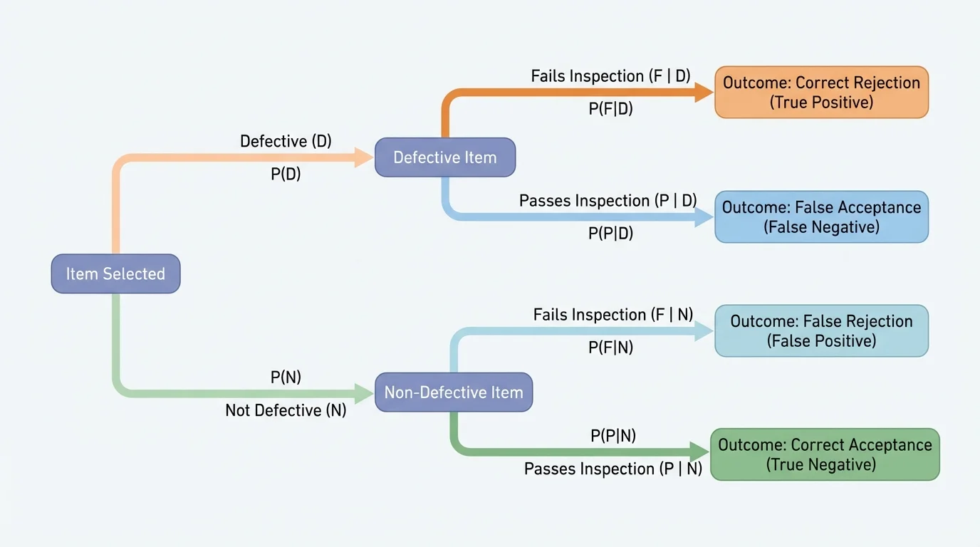
A sample space is the set of all possible outcomes. An event is a collection of outcomes we care about, such as "the test is positive" or "the team ties the game." A tree diagram can organize possibilities with branching outcomes in a testing process. This structure is especially useful when one probability depends on something that happened earlier.
[Figure 1] A conditional probability is the probability of an event given that another event has already occurred. We write it as \(P(A \mid B)\), which means "the probability of \(A\) given \(B\)." In decision-making, this matters because new information can change probabilities. For example, the probability that a person has a disease after testing positive is not the same as the probability of testing positive if the person has the disease.
Two events are independent if one does not affect the probability of the other. If they are independent, then \(P(A \cap B) = P(A)P(B)\). But many real decisions involve events that are not independent. In medical testing, the chance of a positive result depends strongly on whether the person actually has the disease. In product testing, the chance that another item is defective may depend on how the manufacturing process is working that day.
A powerful tool for comparing choices is expected value. Expected value combines probability and outcome size into one number. If an outcome \(x_1\) happens with probability \(p_1\), outcome \(x_2\) with probability \(p_2\), and so on, then the expected value is
\[E = p_1x_1 + p_2x_2 + p_3x_3 + \cdots\]
This does not predict exactly what will happen in one trial. Instead, it gives the average result over many similar situations. In business, expected value can represent average profit or cost. In sports, it can represent expected standings points, chance of advancing, or average goal differential under a strategy.
Expected value is the long-run average outcome of a random process, found by multiplying each outcome by its probability and then adding the results.
Conditional probability is the probability that one event occurs given that another event is known to have occurred.
Complement rule uses the idea that if an event does not happen, its complement does, so \(P(\textrm{not }A) = 1 - P(A)\).
Using the complement is often the quickest way to analyze a decision. If a company wants the probability that at least one sampled item is defective, it may be easier to compute the probability that none are defective and subtract from \(1\). If a team wants the probability of scoring at least once in the final minute, it may be easier to compute the chance of not scoring at all and use the complement.
To analyze a decision, we first define the choices, possible outcomes, and quantities that matter. Sometimes the quantity is money. Sometimes it is patient safety. Sometimes it is the probability of tying a game or winning a championship. Good models are simple enough to calculate but detailed enough to reflect reality.
A useful way to organize a model is with a table of outcomes and probabilities.
| Choice | Possible Outcome | Probability | Value or Cost |
|---|---|---|---|
| Strategy A | Success | \(p\) | \(+V\) |
| Strategy A | Failure | \(1-p\) | \(-C\) |
| Strategy B | Success | \(q\) | \(+W\) |
| Strategy B | Failure | \(1-q\) | \(-D\) |
Table 1. A general structure for comparing decision options by probability and outcome value.
Once the model is built, we compute expected values or specific probabilities. Then we interpret the result in context. A choice with the highest expected profit may not be best if it carries a risk the company cannot afford. A medical strategy with slightly better expected accuracy might still be rejected if it causes too many dangerous false negatives.
Good decisions versus good outcomes
Probability evaluates the quality of a decision based on the information available beforehand. If a basketball player takes a wide-open shot and misses, it was still a good choice because the shot had a high probability of success. Similarly, a doctor or company manager should be evaluated by how reasonable the decision was under uncertainty, not just by whether the outcome turned out well in a single case.
That distinction is one of the most important ideas in applied probability. If people only judge by results, they may abandon strategies that are mathematically sound just because of a short streak of bad luck. Over many trials, probabilities matter more than one dramatic example.
Suppose a factory knows that \(2\%\) of its products are defective. A store receives a large shipment and decides to test a random sample of \(5\) items. The store wants to know the chance that the sample includes at least one defective item. This question affects whether sampling is a useful way to detect problems.
Let \(D\) be the event that a sampled item is defective. Then \(P(D) = 0.02\), and \(P(\textrm{not }D) = 0.98\). Assuming the sampled items are approximately independent, the probability that all \(5\) sampled items are non-defective is \(0.98^5\). Therefore, the probability of at least one defective item is
\[1 - 0.98^5 \approx 1 - 0.9039 = 0.0961\]
So there is about a \(9.61\%\) chance that the sample includes at least one defective item. This is lower than many people expect. If defects are rare, small samples often miss them.
Solved example 1: Deciding whether a sample is large enough
A manufacturer estimates that \(4\%\) of items are defective. A quality-control team tests \(10\) random items. What is the probability that the team finds at least one defective item?
Step 1: Use the complement
It is easier to calculate the probability that no defective items are found. The probability that one item is not defective is \(0.96\).
Step 2: Find the probability that all \(10\) items are not defective
Assuming independence, \(P(\textrm{none defective}) = 0.96^{10} \approx 0.6648\).
Step 3: Subtract from \(1\)
\[P(\textrm{at least one defective}) = 1 - 0.96^{10} \approx 1 - 0.6648 = 0.3352\]
The probability that the sample includes at least one defective item is about \(0.3352\), or \(33.52\%\).
This result can guide action. If a one-third detection chance is too low, the company might test more items, improve production, or use a different rule for accepting a batch. Notice how the probability model helps compare costs: larger samples improve detection but require more time and money.
The tree idea from [Figure 1] also helps in multi-stage inspection systems, where an item may first be sampled and then sent for a more detailed check if the first test raises concerns. At each branch, probabilities combine with decision rules.
[Figure 2] Medical tests are one of the clearest examples of why conditional probability matters. A test can be highly accurate and still produce many misleading positives when the disease is rare. Frequency models make this easier to see by showing how a large population can be split by actual disease status and test result.
Two important measures are often used. Sensitivity is the probability that the test is positive given that the person has the disease. Specificity is the probability that the test is negative given that the person does not have the disease. These are useful, but they do not directly answer the question most patients ask: "If my test is positive, what is the probability that I actually have the disease?" That question is a conditional probability in the other direction, as the population breakdown in the diagram helps illustrate.
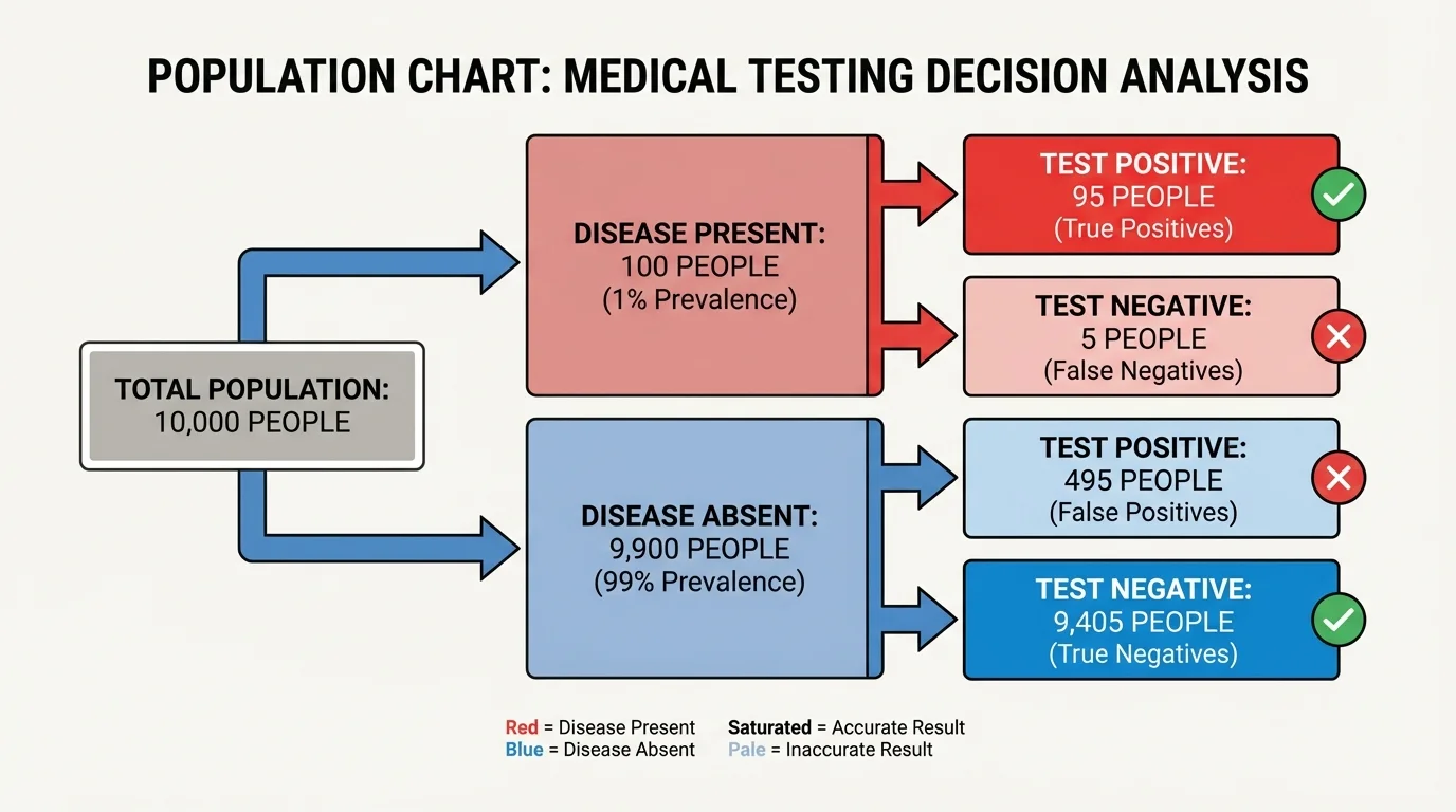
Suppose a disease affects \(1\%\) of a population. A test has sensitivity \(0.95\) and specificity \(0.90\). We test \(10{,}000\) people. About \(100\) have the disease and \(9{,}900\) do not.
Of the \(100\) with the disease, \(95\) test positive. Of the \(9{,}900\) without the disease, \(10\%\) test positive because the specificity is \(0.90\), so \(990\) people without the disease still test positive. That means there are \(95 + 990 = 1{,}085\) positive tests total, but only \(95\) of those are true positives.
Solved example 2: Probability of having a disease after a positive test
Using the situation above, find the probability that a person actually has the disease given a positive result.
Step 1: Identify the number of true positives
True positives: \(95\).
Step 2: Identify the total number of positive tests
Total positives: \(95 + 990 = 1{,}085\).
Step 3: Form the conditional probability
\[P(\textrm{disease} \mid \textrm{positive}) = \frac{95}{1085} \approx 0.0876\]
So the probability is about \(0.0876\), or \(8.76\%\).
This can be surprising. The test seems good, yet a positive result still means the person is more likely not to have the disease than to have it. The reason is the low base rate of the disease in the population. Rare conditions create many opportunities for false positives to outnumber true positives.
Later follow-up testing is often designed to increase confidence by combining information. The population picture in [Figure 2] helps explain why doctors may order a second test instead of acting on one result alone.
A test with excellent sensitivity and specificity can still have a low positive predictive value when the disease is rare. This is one reason screening programs are designed carefully and often target higher-risk groups.
[Figure 3] Near the end of a hockey game, a team that is trailing by one goal sometimes removes its goalie and adds an extra attacker. The diagram helps compare the chances of tying the game and conceding an empty-net goal under the two options. To many fans, this looks reckless, but the strategy depends on probability.
If the team keeps the goalie in net, its chance of scoring may be relatively low. If it pulls the goalie, its chance of scoring rises, but so does the chance of the opponent scoring into the empty net. The key insight is that if the team is already losing late, losing by two instead of one is often not much worse. What matters most is increasing the chance to tie.
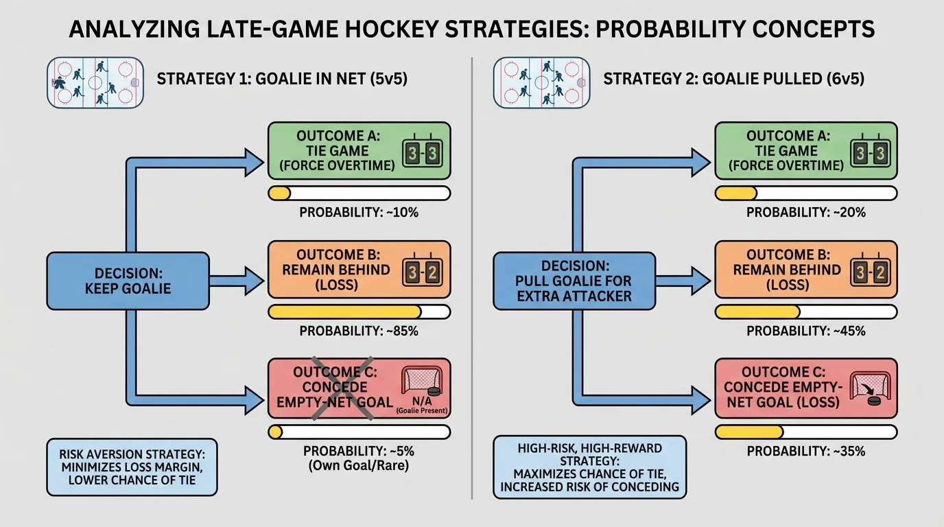
Suppose with \(1\) minute left, a team estimates these probabilities:
| Strategy | Score and tie | Give up goal | No score by either team |
|---|---|---|---|
| Goalie stays | \(0.08\) | \(0.02\) | \(0.90\) |
| Goalie pulled | \(0.18\) | \(0.32\) | \(0.50\) |
Table 2. Estimated late-game probabilities for two hockey strategies.
If the only important objective is to avoid losing by more than one goal, keeping the goalie is better. But if the main goal is to maximize the chance of eventually winning or forcing overtime, the relevant probability is the chance to tie. Then \(0.18 > 0.08\), so pulling the goalie is the better choice.
Solved example 3: Choosing the strategy with the higher chance to continue the game
A team values the outcomes this way: tying the game is worth \(1\), while any loss is worth \(0\). Which strategy has the greater expected value?
Step 1: Define the payoff
Payoff is \(1\) for a tie and \(0\) otherwise.
Step 2: Compute expected value for keeping the goalie
Since only a tie earns value, \(E_{\textrm{stay}} = 1(0.08) + 0(0.92) = 0.08\).
Step 3: Compute expected value for pulling the goalie
Similarly, \(E_{\textrm{pull}} = 1(0.18) + 0(0.82) = 0.18\).
Step 4: Compare
\(0.18 > 0.08\)
Pulling the goalie gives the higher expected value when the goal is to maximize the chance of tying the game.
This is a great example of how probability and goals work together. The "best" strategy depends on what outcome is being optimized. If preserving goal differential matters, the answer may change. If avoiding regulation losses at all costs matters, increasing tie probability may dominate the decision.
Sports analysts often revisit the logic shown in [Figure 3] and compare actual game data with the model. That helps teams decide when to pull the goalie, not just whether to do it.
Expected value is especially useful when different decisions have different rewards and costs. For example, suppose a company can run a product test for \(\$2{,}000\). If the test catches a major defect problem, it avoids an expected loss of \(\$15{,}000\). Suppose the probability of catching such a problem is \(0.12\). Then the expected benefit of the test is \(0.12 \cdot 15{,}000 = 1{,}800\) dollars. Since the test costs \(\$2{,}000\), the net expected value is negative by \(\$200\). Under this model, the company would not choose the test.
But that conclusion could change if the potential loss is underestimated, if public reputation damage matters, or if legal consequences make failures more costly than the simple dollar estimate suggests. This shows that expected value depends not only on probability estimates but also on how outcomes are valued.
Expected value does not guarantee the most common outcome
The expected value can be a long-run average that is not itself one of the actual outcomes. For example, a strategy might have expected gain \(2.4\) goals or \(1.7\) points, even though no single game can end with exactly those values. It is still useful because it summarizes repeated performance.
Sometimes expected value is not the only factor. Decision-makers may also consider risk, which is the chance of very bad outcomes or the variability of results. Two strategies can have the same expected value but very different levels of uncertainty. A cautious hospital may prefer a slightly lower expected benefit if it greatly reduces dangerous false negatives. An investor may reject a gamble with high expected profit if the losses could be disastrous.
No probability model is perfect. Real systems change. Player fatigue affects sports data. Manufacturing machines drift out of calibration. Disease prevalence changes over time and across communities. A model is only as good as its assumptions and data.
Another challenge is estimating probabilities themselves. Sometimes we have strong historical data. Other times we rely on expert judgment. In both cases, we should ask whether conditions are similar enough for past probabilities to apply now.
It is also important to avoid confusing probability with certainty. If a strategy has a \(70\%\) chance of success, it will still fail about \(30\%\) of the time in the long run. That failure does not automatically prove the strategy was wrong. Probability guides decisions under uncertainty; it does not remove uncertainty.
"Probability is not about predicting one future with certainty; it is about comparing uncertain futures wisely."
When used carefully, probability becomes a decision tool. It helps people compare choices, communicate risk, and justify strategies. Whether the context is product testing, medical screening, or end-of-game coaching, the same mathematical ideas appear again and again: define outcomes clearly, estimate probabilities reasonably, connect outcomes to value, and choose the strategy that best matches the goal.