A small change in a number can transform an entire decision table. If every prize in a competition doubles, every payoff in the payoff matrix doubles too. If a photo-editing app cuts brightness values in half, the whole image matrix changes instantly. Matrices are powerful because one simple operation can update many values at once. One of the most important of these operations is multiplying a matrix by a single number.
A matrix organizes numbers into rows and columns, often to represent data, coordinates, transformations, or outcomes. In many applications, we do not want to change the shape of the matrix; we want to change the size of all its values in a consistent way. That is exactly what scalar multiplication does.
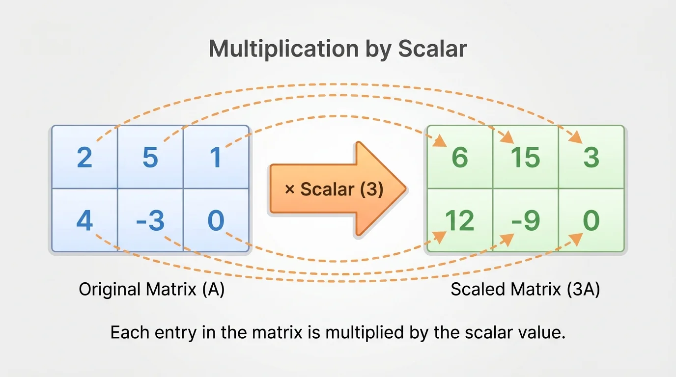
As [Figure 1] suggests, when one number multiplies every entry of a matrix, that number is called a scalar. Scalars are ordinary real numbers such as \(2\), \(-3\), \(0\), or \(\dfrac{1}{2}\). They are different from matrices because a scalar is just a single number.
You already know scalar multiplication from earlier algebra: multiplying a list of numbers by \(k\) means multiplying each number by \(k\). Matrix scalar multiplication uses the same idea, but now the numbers are arranged in rows and columns.
For example, if a matrix stores ticket prices for different sections and days, then multiplying the matrix by \(1.1\) increases all prices by \(10\%\). If a matrix stores the point values in a game, multiplying by \(2\) doubles every reward and penalty. This is why scalar multiplication appears in economics, computer graphics, science, and game theory.
Scalar multiplication takes one number and one matrix and produces a new matrix with the same dimensions. The rule is simple: multiply every entry of the matrix by the same scalar.
If \(A = [a_{ij}]\) is a matrix and \(k\) is a scalar, then the scalar multiple \(kA\) is the matrix whose entries are \(ka_{ij}\).
Scalar multiplication of a matrix means multiplying every entry of a matrix by the same scalar. If \(A = [a_{ij}]\), then
\[kA = [ka_{ij}]\]
The number of rows and columns does not change. Only the entries change.
Suppose
\[A = \begin{bmatrix}1 & -2 & 4 \\ 0 & 3 & 5\end{bmatrix}\]
If we multiply by \(3\), then each entry is multiplied by \(3\):
\[3A = 3\begin{bmatrix}1 & -2 & 4 \\ 0 & 3 & 5\end{bmatrix} = \begin{bmatrix}3 & -6 & 12 \\ 0 & 9 & 15\end{bmatrix}\]
The matrix is still \(2 \times 3\). Scalar multiplication changes values, not size.
Notice that scalar multiplication is an entry-by-entry operation. Every number gets scaled, even if the entry is negative or zero. A negative entry stays negative if multiplied by a positive scalar, but it can change sign if multiplied by a negative scalar.
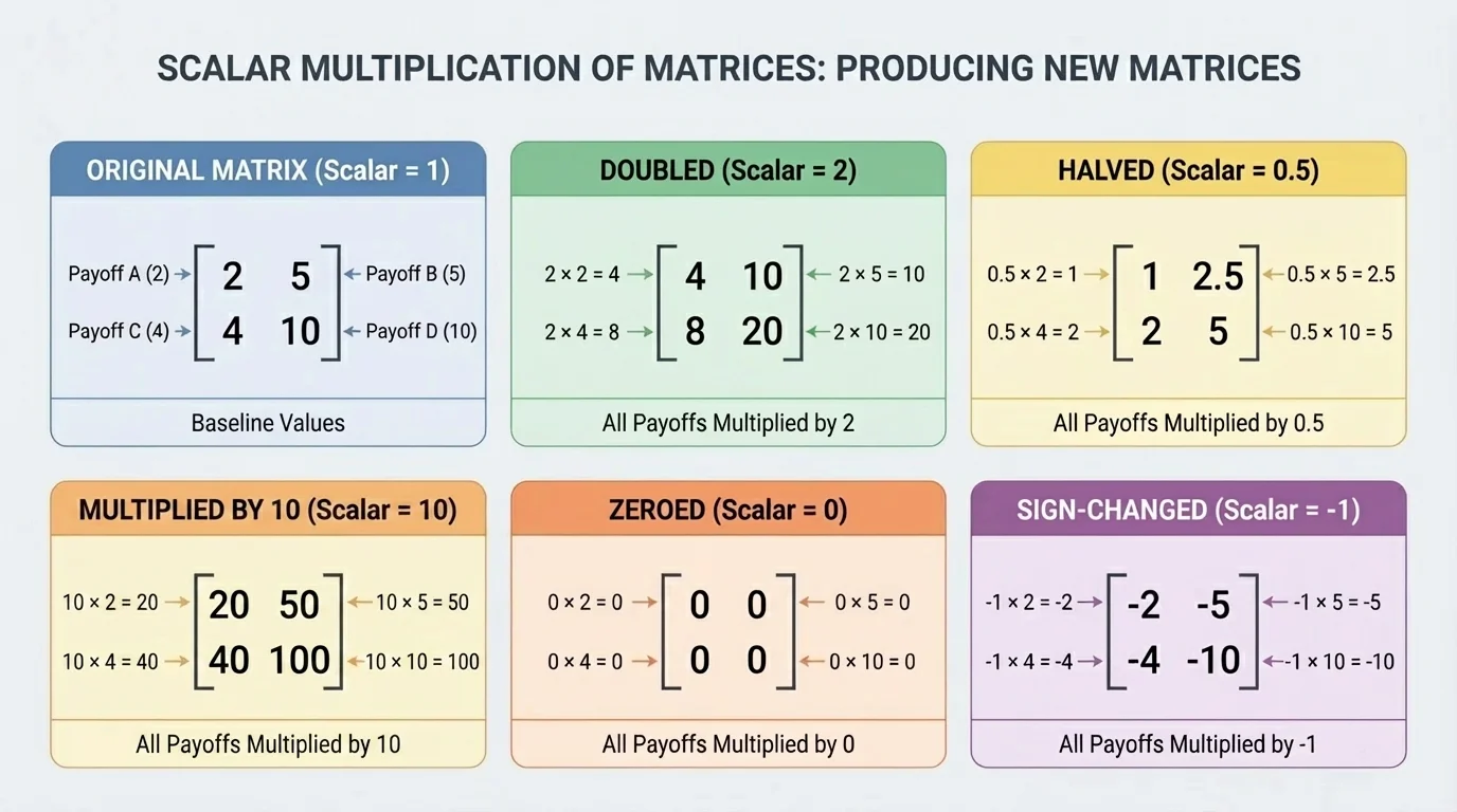
The effect of scaling depends on the scalar itself. As [Figure 2] illustrates, multiplying by different types of scalars can enlarge values, shrink them, reverse signs, or send everything to zero.
If \(k > 1\), then the entries become larger in magnitude. For instance, multiplying by \(2\) doubles each entry. If \(0 < k < 1\), such as \(\dfrac{1}{2}\), the entries become smaller in magnitude. If \(k = 0\), every entry becomes \(0\), producing the zero matrix. If \(k < 0\), then every sign is reversed as well as scaled.
Take the matrix
\[B = \begin{bmatrix}6 & -8 \\ 2 & 10\end{bmatrix}\]
Then:
\[2B = \begin{bmatrix}12 & -16 \\ 4 & 20\end{bmatrix}\]
\[\frac{1}{2}B = \begin{bmatrix}3 & -4 \\ 1 & 5\end{bmatrix}\]
\[-B = \begin{bmatrix}-6 & 8 \\ -2 & -10\end{bmatrix}\]
\[0B = \begin{bmatrix}0 & 0 \\ 0 & 0\end{bmatrix}\]
This matters in interpretation. If a matrix represents profits and losses, multiplying by \(2\) means everything is doubled. If it represents temperatures relative to a baseline, multiplying by \(-1\) flips every value across zero. The numbers change, but the pattern of positions in the matrix remains the same.
Digital images can be stored as grids of numbers. Multiplying all brightness values by a number greater than \(1\) can brighten an image, while multiplying by a number between \(0\) and \(1\) can darken it.
Later, when you study vectors and transformations more deeply, you will see that scalar multiplication is one of the basic operations that makes linear algebra work.
Scalar multiplication follows predictable rules. These properties make calculations more efficient and connect matrix operations to algebra you already know.
Let \(A\) and \(B\) be matrices of the same dimensions, and let \(k\) and \(m\) be scalars.
Identity property: multiplying by \(1\) does not change the matrix.
\(1A = A\)
Zero property: multiplying by \(0\) gives the zero matrix.
\(0A = 0\)
Opposite property: multiplying by \(-1\) gives the additive inverse.
\((-1)A = -A\)
Associative property of scalars: scaling by \(m\) and then by \(k\) is the same as scaling once by \(km\).
\[k(mA) = (km)A\]
Distributive property over matrix addition:
\[k(A + B) = kA + kB\]
Distributive property over scalar addition:
\[(k + m)A = kA + mA\]
These rules are extremely useful. They let us simplify expressions with matrices just as we simplify algebraic expressions with variables.
| Property | Example |
|---|---|
| Identity | \(1A = A\) |
| Zero | \(0A = 0\) |
| Opposite | \((-1)A = -A\) |
| Associative with scalars | \(2(3A) = 6A\) |
| Distributive over matrix addition | \(4(A+B)=4A+4B\) |
| Distributive over scalar addition | \((2+5)A=2A+5A\) |
Table 1. Main properties of matrix scalar multiplication.
These properties also show why scalar multiplication fits naturally with matrix addition. Together, they allow us to build new matrices from combinations of old ones.
Working through examples carefully is the best way to master the procedure. The key habit is always the same: multiply each entry, check the signs, and keep the dimensions unchanged.
Example 1: Multiply a matrix by a positive integer
Find \(4C\) if
\[C = \begin{bmatrix}2 & -1 \\ 5 & 3\end{bmatrix}\]
Step 1: Apply the scalar to each entry.
Multiply \(2\), \(-1\), \(5\), and \(3\) each by \(4\).
Step 2: Compute each new entry.
\(4 \cdot 2 = 8\), \(4 \cdot (-1) = -4\), \(4 \cdot 5 = 20\), and \(4 \cdot 3 = 12\).
Step 3: Write the result in the same shape.
\[4C = \begin{bmatrix}8 & -4 \\ 20 & 12\end{bmatrix}\]
The matrix remains \(2 \times 2\).
This first example shows the basic pattern. Nothing moves to a new position; only the values are scaled.
Example 2: Multiply by a negative fraction
Find \(-\dfrac{1}{2}D\) if
\[D = \begin{bmatrix}8 & -6 & 0 \\ -4 & 10 & 2\end{bmatrix}\]
Step 1: Multiply each entry by \(-\dfrac{1}{2}\).
This means each entry is halved and its sign is reversed.
Step 2: Compute each result.
\((-\dfrac{1}{2})(8) = -4\), \((-\dfrac{1}{2})(-6) = 3\), \((-\dfrac{1}{2})(0)=0\), \((-\dfrac{1}{2})(-4)=2\), \((-\dfrac{1}{2})(10)=-5\), and \((-\dfrac{1}{2})(2)=-1\).
Step 3: Write the new matrix.
\[-\frac{1}{2}D = \begin{bmatrix}-4 & 3 & 0 \\ 2 & -5 & -1\end{bmatrix}\]
Negative and fractional scalars are handled the same way as whole-number scalars: one entry at a time.
Notice how the zero entry stayed zero. That always happens, no matter what scalar is used.
Example 3: Double every payoff in a game
A business game has the payoff matrix
\[P = \begin{bmatrix}3 & -1 \\ 5 & 2\end{bmatrix}\]
If every payoff is doubled, find the new matrix.
Step 1: Identify the scalar.
"Doubled" means multiply by \(2\).
Step 2: Multiply each entry by \(2\).
\(2 \cdot 3 = 6\), \(2 \cdot (-1) = -2\), \(2 \cdot 5 = 10\), and \(2 \cdot 2 = 4\).
Step 3: Write the new payoff matrix.
\[2P = \begin{bmatrix}6 & -2 \\ 10 & 4\end{bmatrix}\]
Each strategy combination now gives twice the original reward or penalty.
This kind of scaling often appears in economics and decision-making. If all rewards and losses are measured in larger units, the payoff matrix scales exactly as shown in [Figure 2].
Example 4: Use a property with addition
Let
\[A = \begin{bmatrix}1 & 2 \\ 0 & -1\end{bmatrix}, \quad B = \begin{bmatrix}3 & -4 \\ 5 & 2\end{bmatrix}\]
Find \(2(A+B)\).
Step 1: Add the matrices.
\[A+B = \begin{bmatrix}1+3 & 2+(-4) \\ 0+5 & -1+2\end{bmatrix} = \begin{bmatrix}4 & -2 \\ 5 & 1\end{bmatrix}\]
Step 2: Multiply the result by \(2\).
\[2(A+B) = 2\begin{bmatrix}4 & -2 \\ 5 & 1\end{bmatrix} = \begin{bmatrix}8 & -4 \\ 10 & 2\end{bmatrix}\]
Step 3: Check with the distributive property.
\[2A = \begin{bmatrix}2 & 4 \\ 0 & -2\end{bmatrix}, \quad 2B = \begin{bmatrix}6 & -8 \\ 10 & 4\end{bmatrix}\]
Then
\[2A + 2B = \begin{bmatrix}8 & -4 \\ 10 & 2\end{bmatrix}\]
Both methods agree, confirming that \(2(A+B)=2A+2B\).
Examples like this show that scalar multiplication is not isolated; it works together with other matrix operations in a consistent algebraic system.
One common error is multiplying only one row or one column by the scalar. Scalar multiplication must affect every entry in the matrix.
Another mistake is confusing scalar multiplication with matrix multiplication. In scalar multiplication, one factor is a single number. In matrix multiplication, both factors are matrices, and the rule is much more complicated. You do not multiply corresponding entries in ordinary matrix multiplication the way you do here.
A third mistake is trying to add the scalar to every entry instead of multiplying. For example, if the scalar is \(3\), then
\[3\begin{bmatrix}1 & 2 \\ 3 & 4\end{bmatrix} = \begin{bmatrix}3 & 6 \\ 9 & 12\end{bmatrix}\]
not
\[\begin{bmatrix}4 & 5 \\ 6 & 7\end{bmatrix}\]
Checking signs is also important. If the scalar is negative, every sign must be handled carefully. A quick mental check can help: multiplying by a negative should reverse the sign of each nonzero entry.
Why the dimensions do not change
Scalar multiplication changes the value of each entry, but it does not add or remove rows and columns. If a matrix starts as \(m \times n\), then \(kA\) is also \(m \times n\). This makes scalar multiplication useful when the arrangement of data must stay fixed while the scale changes.
This is one reason matrices are so practical for modeling. You can update a whole system without changing its structure.
In decision theory and economics, payoff tables are often written as matrices. As [Figure 3] shows, if every possible reward in a game is doubled, then the entire payoff matrix is multiplied by \(2\). The strategy layout stays the same while each outcome is scaled.
Suppose two companies each choose either a high-price or low-price strategy, and the profit matrix for one company is
\[M = \begin{bmatrix}4 & 1 \\ -2 & 3\end{bmatrix}\]
If market demand increases so that all profits and losses are doubled, the new matrix is
\[2M = \begin{bmatrix}8 & 2 \\ -4 & 6\end{bmatrix}\]
The strategic structure does not change, but the size of every consequence does.

Matrices can also represent data tables. If a school tracks energy use in several buildings over several months, and the numbers are converted from one unit to another, the whole matrix may be multiplied by a conversion factor. In science, measurement arrays are often scaled this way.
In computer graphics, a grayscale image can be represented by a matrix of brightness values. Multiplying all entries by \(1.2\) makes the image brighter, while multiplying by \(0.8\) makes it dimmer. In that setting, the location of each pixel stays fixed, just as rows and columns stay fixed in a matrix.
In physics, vectors and matrices often describe quantities such as position, force, or data collected over time. If all measurements are converted from meters to centimeters, each value is multiplied by \(100\). The same mathematical idea appears again and again because scaling is fundamental.
The game-payoff example also helps explain why scalar multiplication is useful in analysis. Instead of recalculating every strategic option separately, one multiplication updates the entire table at once.
Scalar multiplication combines naturally with matrix addition and subtraction. In fact, many matrix expressions are built from linear combinations, which are sums of scalar multiples of matrices.
For example, if
\(X = 2A - 3B\)
then \(X\) is made by scaling \(A\) by \(2\), scaling \(B\) by \(-3\), and then subtracting. This kind of expression appears throughout algebra, geometry, economics, and data science.
Returning to the earlier visual model in [Figure 1], the important idea is that a scalar acts uniformly on the whole matrix. That uniformity is what makes matrix algebra organized and predictable.
Once you are comfortable with scalar multiplication, you are ready to use matrices more flexibly: adding them, subtracting them, and combining them into larger models of real systems.