One of the most powerful ideas in algebra is that some processes can be reversed. If a machine triples a number and then adds \(5\), you can work backward to recover the original input. In mathematics, that "working backward" idea becomes especially important when solving equations like \(f(x)=c\). Instead of attacking the equation from scratch every time, you can use the inverse of the function to undo what \(f\) does.
When you solve an equation such as \(2x+7=15\), you are already using inverse operations: subtract \(7\), then divide by \(2\). Inverse functions extend that same idea to entire functions. If a function is reversible, then solving \(f(x)=c\) is often as simple as applying the inverse function to both sides and getting \(x=f^{-1}(c)\).
This matters far beyond textbook algebra. A formula may tell you the output from an input, but in science, engineering, economics, and technology, you often need the reverse question: given the output, what was the input? That is exactly what inverse functions help you answer.
From earlier algebra, you already know how to undo operations: addition is undone by subtraction, multiplication by division, powers by roots when appropriate, and fractions by inverse algebraic steps. Inverse functions package those undoing steps into a single new function.
To use an inverse function correctly, the original function must be reversible on its domain. That means each output comes from exactly one input.
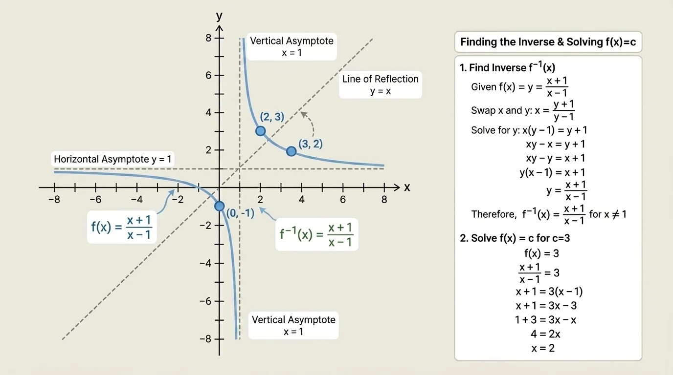
A inverse function reverses the action of another function. If \(f\) takes \(x\) to \(y\), then \(f^{-1}\) takes \(y\) back to \(x\). [Figure 1] Graphically, the function and its inverse are reflections across the line \(y=x\).
If \(f(a)=b\), then the inverse relationship is \(f^{-1}(b)=a\). These two statements mean the same pairing, just read in opposite directions.
Not every function has an inverse that is also a function. For that to happen, the original function must be one-to-one. A function is one-to-one if different inputs always produce different outputs. In graph terms, it passes the horizontal line test: every horizontal line intersects the graph at most once.
For example, \(f(x)=x^2\) is not one-to-one on all real numbers because \(f(2)=4\) and \(f(-2)=4\). But if the domain is restricted to \(x\ge 0\), then the function becomes one-to-one and has inverse \(f^{-1}(x)=\sqrt{x}\).
Inverse function means a function that undoes another function. If \(f^{-1}\) is the inverse of \(f\), then \(f(f^{-1}(x))=x\) for inputs in the domain of \(f^{-1}\), and \(f^{-1}(f(x))=x\) for inputs in the domain of \(f\).
The notation \(f^{-1}(x)\) does not mean \(\dfrac{1}{f(x)}\). It means the inverse function. That notation is easy to confuse at first, so it is worth paying attention to context.
Suppose \(f\) is invertible and you want to solve
\(f(x)=c\)
If you apply the inverse function to both sides, you get
\[f^{-1}(f(x))=f^{-1}(c)\]
Since \(f^{-1}\) undoes \(f\), this simplifies to
\(x=f^{-1}(c)\)
This is the main idea of the lesson: to solve \(f(x)=c\), apply the inverse function and compute \(x=f^{-1}(c)\).
However, there is an important detail. The value \(c\) must be in the range of \(f\). If \(c\) is not an output of the function, then the equation has no solution.
To find an inverse function algebraically, there is a standard method. It works for many common functions.
Step 1: Write \(y=f(x)\).
Step 2: Swap \(x\) and \(y\). This reflects the input-output roles.
Step 3: Solve for \(y\).
Step 4: Rename \(y\) as \(f^{-1}(x)\).
This process works because if \(f\) sends \(x\) to \(y\), then the inverse sends \(y\) back to \(x\).
Why swapping \(x\) and \(y\) works
In a function, \(x\) is the input and \(y\) is the output. For the inverse, those roles switch. A point \((a,b)\) on the graph of \(f\) becomes the point \((b,a)\) on the graph of \(f^{-1}\). That is why interchanging \(x\) and \(y\) is the algebraic heart of the inverse process.
After finding an inverse, you should check it by composition. If your answer is correct, then composing the function and its inverse returns the original input.
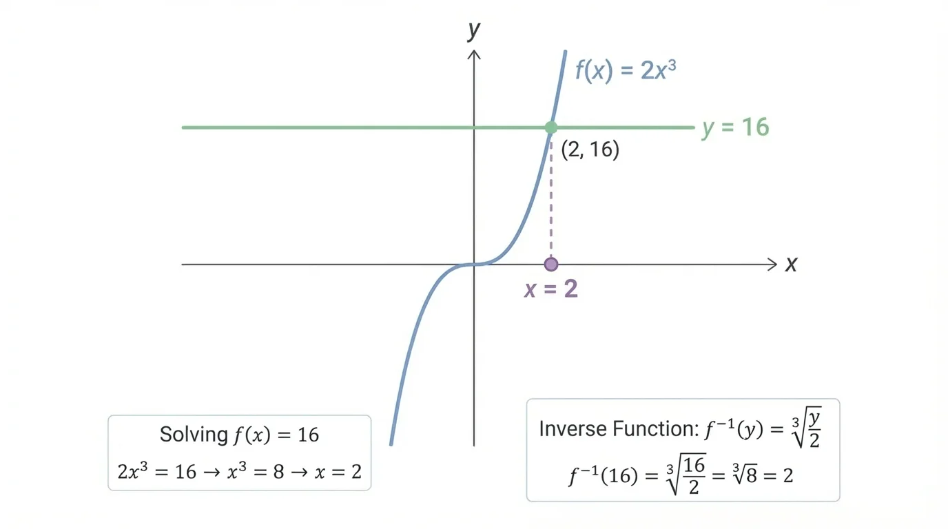
Consider the function \(f(x)=2x^3\). This function is one-to-one on all real numbers, so it has an inverse. It also has exactly one solution to \(f(x)=c\) for any real number \(c\), which the graph makes visible through a single intersection with a horizontal line, as [Figure 2] illustrates.
We will do two things: solve \(f(x)=c\), and then find a formula for \(f^{-1}(x)\).
Worked example: solve \(2x^3=c\) and find the inverse
Step 1: Solve the equation \(f(x)=c\).
Start with \(2x^3=c\). Divide both sides by \(2\): \(x^3=\dfrac{c}{2}\). Then take the cube root of both sides: \(x=\sqrt[3]{\dfrac{c}{2}}\).
Step 2: Find the inverse algebraically.
Let \(y=2x^3\). Swap \(x\) and \(y\): \(x=2y^3\). Solve for \(y\): \(y^3=\dfrac{x}{2}\), so \(y=\sqrt[3]{\dfrac{x}{2}}\).
Step 3: Write the inverse function.
\[f^{-1}(x)=\sqrt[3]{\frac{x}{2}}\]
Step 4: Verify by composition.
Compute \(f(f^{-1}(x))=2\left(\sqrt[3]{\dfrac{x}{2}}\right)^3=2\cdot \dfrac{x}{2}=x\).
So the solution to \(f(x)=c\) is \(x=\sqrt[3]{\dfrac{c}{2}}\), and the inverse is \(f^{-1}(x)=\sqrt[3]{\dfrac{x}{2}}\).
Notice how solving the equation and finding the inverse are closely connected. Once you know the inverse, the solution to \(f(x)=c\) is immediate: just plug \(c\) into \(f^{-1}\).
The graph in [Figure 2] also reinforces an important idea: because the cubic function keeps increasing, every horizontal line hits it exactly once. That is why the inverse exists for all real inputs and outputs.
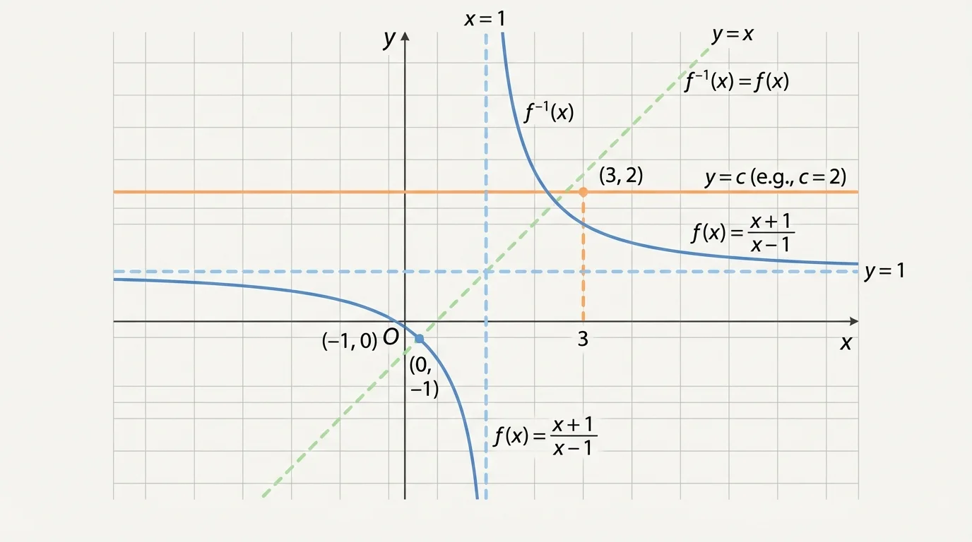
[Figure 3] Now consider a rational function: \(f(x)=\dfrac{x+1}{x-1}\), with domain \(x\ne 1\). This is a richer example because the function has a restriction, and its graph has asymptotes. Those asymptotes help explain why some values are excluded.
We first ask: what happens when we solve \(\dfrac{x+1}{x-1}=c\)?
Worked example: solve \(\dfrac{x+1}{x-1}=c\)
Step 1: Start with the equation.
\(\dfrac{x+1}{x-1}=c\)
Step 2: Multiply both sides by \(x-1\).
\(x+1=c(x-1)\)
Step 3: Expand and collect \(x\)-terms.
\(x+1=cx-c\). Move the \(x\)-terms together: \(x-cx=-c-1\).
Step 4: Factor and solve.
\(x(1-c)=-(c+1)\), so \(x=\dfrac{-(c+1)}{1-c}\). Multiplying top and bottom by \(-1\) gives \(x=\dfrac{c+1}{c-1}\).
Therefore, when \(c\ne 1\), the solution is \[x=\frac{c+1}{c-1}\]
Why must \(c\ne 1\)? If we try \(\dfrac{x+1}{x-1}=1\), then we get \(x+1=x-1\), which simplifies to \(1=-1\), impossible. So \(1\) is not in the range of the function.
That means the inverse function will also have a restriction: its domain cannot include \(1\). This matches the graph, where the horizontal asymptote is \(y=1\), and the curve never actually reaches that value.
Now let us find the inverse formula itself.
Worked example: find the inverse of \(f(x)=\dfrac{x+1}{x-1}\)
Step 1: Write \(y=\dfrac{x+1}{x-1}\).
Step 2: Swap \(x\) and \(y\).
\(x=\dfrac{y+1}{y-1}\)
Step 3: Solve for \(y\).
Multiply both sides by \(y-1\): \(x(y-1)=y+1\). Expand: \(xy-x=y+1\). Collect \(y\)-terms: \(xy-y=x+1\). Factor: \(y(x-1)=x+1\). So \(y=\dfrac{x+1}{x-1}\).
Step 4: Write the inverse.
\[f^{-1}(x)=\frac{x+1}{x-1}, \quad x\ne 1\]
This function is its own inverse. That means applying it twice returns you to your starting value.
Functions that are their own inverses are especially interesting. They have a kind of built-in symmetry. Algebraically, this one returns to itself after the swap-and-solve process.
Inverse problems do not always look the same, but the main ideas stay consistent. Here are a few important variations.
Restricted-domain square function: Suppose \(f(x)=x^2\) with domain \(x\ge 0\). To solve \(f(x)=c\), you solve \(x^2=c\). Since the domain only allows nonnegative \(x\), the solution is \(x=\sqrt{c}\), provided \(c\ge 0\). The inverse is \(f^{-1}(x)=\sqrt{x}\).
Linear function: If \(f(x)=3x-4\), then solving \(f(x)=c\) gives \(3x-4=c\), so \(x=\dfrac{c+4}{3}\). The inverse is \(f^{-1}(x)=\dfrac{x+4}{3}\).
A common mistake: forgetting domain and range restrictions. If a function excludes certain inputs, the inverse excludes the corresponding outputs. For the rational example, the original function excludes \(x=1\), and the inverse excludes \(x=1\) as well, but these restrictions come from different roles: one is a domain restriction for the original function, and the other is a domain restriction for the inverse because \(1\) is not in the original range.
Some functions are not invertible on their full domains but become invertible after a carefully chosen restriction. This is why trigonometric inverses such as \(\sin^{-1}(x)\) require a restricted domain for sine.
Another common mistake is assuming every equation \(f(x)=c\) has a solution. That only happens when \(c\) is actually in the range of \(f\). For example, with \(f(x)=x^2\) on the domain \(x\ge 0\), the equation \(f(x)=-9\) has no real solution because \(x^2\) is never negative.
Once you find an inverse, it is good algebraic practice to verify it. The standard checks are
\[f(f^{-1}(x))=x\]
and
\[f^{-1}(f(x))=x\]
as long as the inputs are in the appropriate domains.
For the cubic example, we already checked one composition. Let us check the rational example quickly:
\(f(f(x))=\dfrac{\dfrac{x+1}{x-1}+1}{\dfrac{x+1}{x-1}-1}\).
Simplifying the numerator gives \(\dfrac{x+1+x-1}{x-1}=\dfrac{2x}{x-1}\). Simplifying the denominator gives \(\dfrac{x+1-(x-1)}{x-1}=\dfrac{2}{x-1}\). So
\(f(f(x))=\dfrac{\dfrac{2x}{x-1}}{\dfrac{2}{x-1}}=x\), for \(x\ne 1\).
This confirms that the function really is its own inverse.
Equation solving and inverse functions are two views of the same idea
When you solve \(f(x)=c\), you are asking which input produces the output \(c\). The inverse function answers that question directly by sending \(c\) back to its original input. In this way, inverse functions turn equation solving into function evaluation.
That connection is one reason inverse functions are so useful. They make many repeated solving tasks faster and more organized.
Inverse functions appear whenever a situation involves encoding and decoding, converting and reversing, or finding an original input from a measured output.
Engineering and science: A formula may describe how an instrument converts a physical quantity into a reading. If the device output is known, the inverse recovers the actual quantity being measured.
Temperature conversion: If \(F=\dfrac{9}{5}C+32\), then the inverse gives Celsius from Fahrenheit: \(C=\dfrac{5}{9}(F-32)\). That is an inverse function in action.
Computer graphics and scaling: If a screen program transforms coordinates using a function, the inverse can restore the original coordinates. Reversible transformations are essential when zooming, rotating, or mapping points between systems.
Economics: A business might know revenue as a function of items sold, but to meet a target revenue, it must solve for how many items need to be sold. If the function is invertible, the inverse provides the answer directly.
Worked example: a real-world linear inverse
A delivery service models total cost by \(C(n)=5n+12\), where \(n\) is the number of packages and \(C(n)\) is the total cost in dollars.
Step 1: Solve \(C(n)=c\) for \(n\).
Start with \(5n+12=c\). Then \(5n=c-12\), so \(n=\dfrac{c-12}{5}\).
Step 2: Write the inverse.
\[C^{-1}(x)=\frac{x-12}{5}\]
Step 3: Interpret it.
If the total cost is 47 dollars, then \(n=C^{-1}(47)=\dfrac{47-12}{5}=7\). So the charge corresponds to \(7\) packages.
The same logic works in more advanced mathematics too. As functions become more complex, the inverse idea remains the same: reverse the process, respect the domain and range, and verify the result.
If a function is invertible, then solving \(f(x)=c\) becomes a clear procedure: apply \(f^{-1}\) and get \(x=f^{-1}(c)\). That sounds simple, but behind it are several essential ideas: the function must be one-to-one, the value \(c\) must lie in the range, and restrictions must be handled carefully.
As you continue studying algebra and beyond, this topic becomes a bridge between equation solving, graphing, and function thinking. It is one of the places where algebra becomes more than symbol manipulation: it becomes a way of understanding reversible relationships.