A movie reviewer does not need to watch every second of every film ever made to notice trends, and scientists do not test every leaf in a forest to study a disease. In the same way, statisticians often learn about a large group by studying a smaller part of it. That idea is powerful, but it comes with a challenge: a small sample can help us make a smart estimate, yet it will almost never match the whole population exactly.
A population is the entire group we want to learn about. It might be all the students in a school, all the words in a book, or all the cans coming off a factory line in one day. A sample is a smaller group chosen from the population.
Sampling is useful because studying a whole population may take too much time, cost too much money, or simply be impossible. If you want to estimate the average length of words in a novel, counting every word would be slow. If you want to predict the winner of a school election, asking every student before the election may not work. A sample gives a practical way to gather information.
Population means the full group being studied. Sample means part of that group. An inference is a conclusion about the population based on the sample data.
The main goal is to use sample data to make an inference about the larger population. For example, if the average word length in your sample is about \(4.6\) letters, you may infer that the average word length in the whole book is close to \(4.6\) letters. If \(52\) out of \(100\) randomly surveyed students prefer one candidate, you may infer that candidate might win the election.
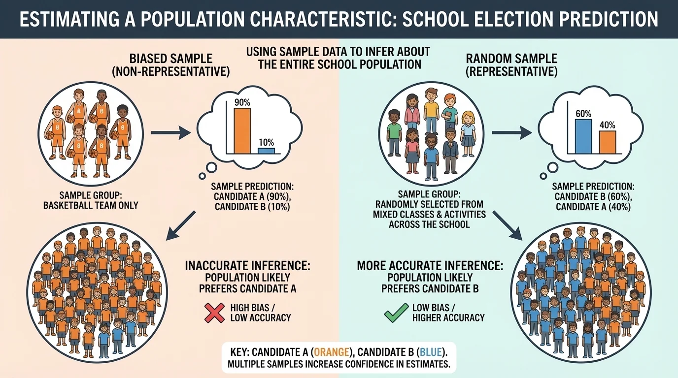
A random sample is chosen so that every member of the population has a fair chance of being selected. This matters because a random sample is more likely to represent the whole population well, as [Figure 1] illustrates when comparing a balanced school sample with a sample drawn from only one group.
If a sample is not chosen fairly, it may be biased. A biased sample tends to favor one part of the population and can lead to misleading conclusions. For example, if you survey only students leaving the gym to predict the favorite school sport, your results may not represent the entire school.
Random does not mean messy or careless. It means the selection follows a fair method. You might number all students and use a random number generator, pull names from a container, or choose every \(10\)th item after a random starting point. These methods help reduce bias.
Even a random sample is not perfect. It gives useful information, but there can still be differences between the sample and the population. That is why statisticians think carefully about variation, not just one answer.
To find an average, add the values and divide by the number of values. In statistics, this average is often called the mean. To find a proportion, divide the number with a certain result by the total number in the sample.
Suppose a sample of \(20\) words has a total of \(92\) letters. The sample mean word length is \(\dfrac{92}{20} = 4.6\) letters. If a sample of \(80\) students includes \(44\) who support Candidate A, the sample proportion for Candidate A is \(\dfrac{44}{80} = 0.55\), or \(55\%\).
When we use a sample to say something about a population, we are estimating an unknown characteristic. Sometimes the characteristic is a mean, such as average height, average score, or average word length. Sometimes it is a proportion, such as the fraction of students who prefer pizza or the fraction of voters who support a candidate.
To estimate a population mean, we often use the sample mean. To estimate a population proportion, we often use the sample proportion. These are not guaranteed to be exact, but they are reasonable estimates when the sample is random and large enough.
Estimate versus exact answer
An estimate is a value that is likely to be close to the true population value. Because it comes from a sample, it may be a little high or a little low. The key idea is not that the estimate is perfect, but that it is useful and based on evidence.
For example, if you randomly sample words from a book and get an average of \(4.6\) letters, you should not claim the exact mean word length of the entire book is definitely \(4.6\). A better statement is that the population mean is probably near \(4.6\) letters.
Likewise, if \(55\%\) of a random sample of students support Candidate A, you might predict that Candidate A will win. But you should also remember that another random sample might give \(52\%\) or \(58\%\). Sampling gives evidence, not certainty.
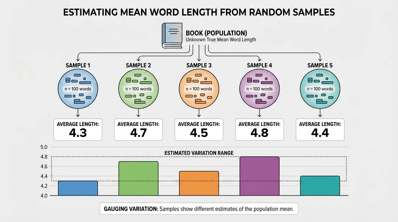
One of the most important ideas in statistics is variation. As [Figure 2] shows, if you take several random samples of the same size from the same population, the results will usually be similar but not identical.
This happens because each sample contains different members of the population. A sample of \(20\) words from a book might happen to include more short words, while another sample of \(20\) words might include more long words. A survey of \(100\) students might happen to include slightly more supporters of one candidate than another equally fair sample.
Variation is not a mistake. It is a normal part of sampling. In fact, understanding this variation helps us judge how reliable an estimate is. If repeated samples stay close together, we feel more confident. If they spread out a lot, we know the estimate can vary more.
Sample size matters too. In general, larger random samples tend to give more stable estimates than smaller ones. A sample of \(200\) students usually gives a more dependable election estimate than a sample of \(20\) students, because the larger sample is less affected by a few unusual choices.
Political polls often report that results may be off by a few percentage points. That idea comes from the fact that different random samples can give slightly different results, even when the poll is conducted carefully.
Think of tossing a coin. If you toss it \(10\) times, getting \(7\) heads is possible. If you toss it \(1{,}000\) times, the proportion of heads is usually much closer to \(0.5\). Sampling works in a similar way: more data usually means less variation in the estimate.
To understand how far off an estimate or prediction might be, we can generate multiple samples of the same size. These can be real samples or simulated samples made with technology, random digits, or repeated draws from a model.
Suppose you want to estimate average word length in a long book. You could take one random sample of \(25\) words and get \(4.4\). But if you take several random samples of \(25\) words, you might get means like \(4.2\), \(4.6\), \(4.5\), \(4.3\), and \(4.7\). That tells you the true mean is probably near the middle of those values, and a single estimate of \(4.4\) is likely to be off by only a few tenths, not by whole letters.
Now consider an election survey. If several random samples of \(100\) students give Candidate A support levels of \(51\%\), \(54\%\), \(52\%\), \(55\%\), and \(53\%\), then A seems likely to be ahead. But if the sample results are \(49\%\), \(52\%\), \(50\%\), \(48\%\), and \(51\%\), the race seems much less certain.
Using repeated samples to gauge uncertainty
Repeated sampling helps answer a practical question: How much could my estimate change if I sampled again? If the answers from many samples stay in a narrow range, the estimate is more stable. If they spread out widely, the estimate is less certain.
This is why statisticians do not focus only on one number. They also pay attention to the likely spread of results from many samples of the same size.
You can use a sample mean to estimate a population mean. Here, the population is all words in a book, and the sample contains randomly chosen words from that book.
Worked example
A student randomly samples \(12\) words from a book. Their lengths are \(3, 5, 4, 6, 4, 7, 5, 4, 3, 6, 5, 4\). Estimate the mean word length in the book.
Step 1: Add the word lengths.
\(3 + 5 + 4 + 6 + 4 + 7 + 5 + 4 + 3 + 6 + 5 + 4 = 56\)
Step 2: Divide by the number of words.
There are \(12\) words, so the sample mean is \(\dfrac{56}{12}\).
\(\dfrac{56}{12} = 4.666\ldots\)
Step 3: Round to a sensible estimate.
The sample mean is about \(4.7\) letters.
The estimated mean word length in the book is \(4.7\) letters.
This does not prove that every chapter in the book has the same average. It means that, based on this random sample, \(4.7\) letters is a reasonable estimate for the population mean.
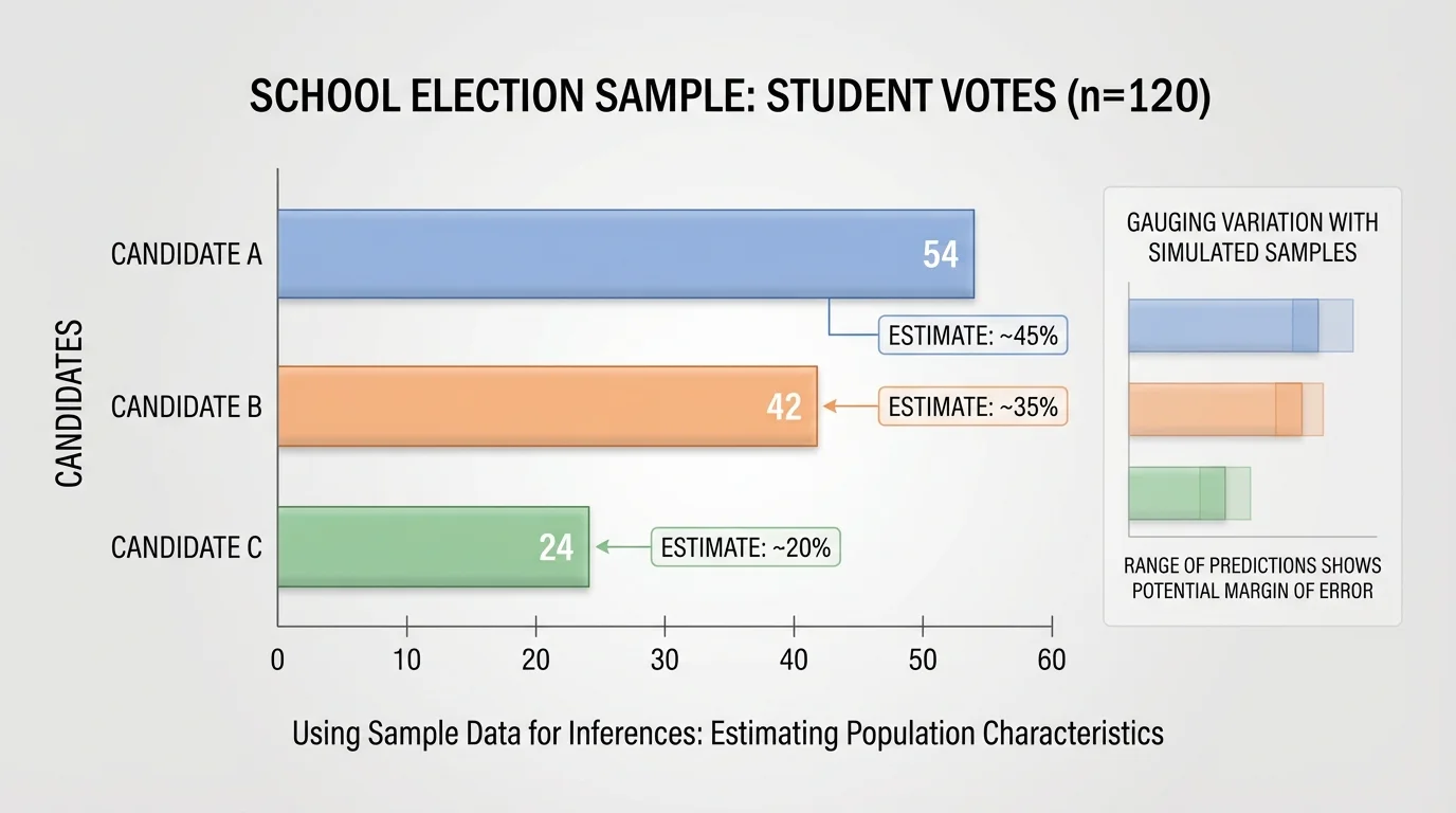
When a sample measures support for candidates, the sample proportions can be compared visually, as [Figure 3] helps show, and the candidate with the highest support in the sample is the most likely winner.
Suppose a random survey of students is taken before the election. The goal is not to know the exact final result yet, but to use sample evidence to make a prediction.
Worked example
In a random sample of \(120\) students, \(54\) support Candidate A, \(42\) support Candidate B, and \(24\) support Candidate C. Predict the winner.
Step 1: Find each sample proportion.
Candidate A: \(\dfrac{54}{120} = 0.45 = 45\%\)
Candidate B: \(\dfrac{42}{120} = 0.35 = 35\%\)
Candidate C: \(\dfrac{24}{120} = 0.20 = 20\%\)
Step 2: Compare the proportions.
\(45\% > 35\% > 20\%\), so Candidate A has the greatest support in the sample.
Step 3: Make a cautious prediction.
Based on the sample, Candidate A is the predicted winner.
The prediction is that Candidate A is most likely to win.
A prediction is strongest when one candidate leads by a comfortable amount. A lead of \(45\%\) to \(35\%\) is more convincing than a lead of \(51\%\) to \(49\%\), because small differences can change from sample to sample.
Later, when discussing uncertainty, we can notice that the sample points to Candidate A, but it still does not guarantee the final election result.
Looking at several samples of the same size helps us estimate not only a center but also the likely amount of variation.
Worked example
Five random samples of \(20\) words are taken from the same book. Their mean word lengths are \(4.2\), \(4.5\), \(4.4\), \(4.7\), and \(4.3\). What can we infer?
Step 1: Look for the center of the sample means.
These values cluster near \(4.4\) to \(4.5\).
Step 2: Look for the spread.
The smallest sample mean is \(4.2\), and the largest is \(4.7\).
The spread across these results is \(4.7 - 4.2 = 0.5\).
Step 3: Make an inference.
A reasonable estimate for the population mean is about \(4.4\) or \(4.5\) letters, and a single sample of size \(20\) might differ by a few tenths of a letter.
A reasonable conclusion is that the population mean is likely near \(4.4\) to \(4.5\).
Notice that none of the sample means are exactly the same. This is the variation we expect from repeated random sampling, just as we saw earlier in [Figure 2].
At this level, you do not need a complicated formula to talk about uncertainty. Instead, use repeated samples to describe a reasonable range. If many sample means are between \(4.3\) and \(4.6\), then an estimate near the middle is sensible, and being off by more than \(0.5\) seems less likely.
For predictions, pay attention to how much one result leads another. If repeated election samples almost always show Candidate A ahead, the prediction is fairly strong. If some samples show A ahead and others show B ahead, the race is too close to call with confidence.
"A sample gives evidence, not certainty."
This idea also explains why a single dramatic sample can be misleading. If one survey of \(20\) students shows \(70\%\) support for a candidate, that sounds impressive. But another sample of \(20\) might give a very different result. A larger sample, or several samples, gives a clearer picture.
Sampling is everywhere. Doctors use samples in medical studies. Companies test sample products for quality. Ecologists sample parts of forests, lakes, or animal populations. Sports analysts use sample statistics from games to estimate a player's typical performance.
Suppose a company checks \(50\) light bulbs from a day's production instead of all \(10{,}000\). If \(2\) are defective, the sample defect rate is \(\dfrac{2}{50} = 0.04 = 4\%\). The company may infer that about \(4\%\) of the day's production is defective, though the exact population rate may be somewhat different.
Or suppose a streaming service wants to know the average length of songs users finish listening to. It can randomly sample listening sessions instead of studying every single one. The same reasoning applies: random samples support useful inferences, but repeated samples help reveal how much those estimates might vary.
| Situation | Population | Sample | Possible Inference |
|---|---|---|---|
| Book study | All words in a book | Randomly chosen words | Estimate mean word length |
| School election | All student voters | Randomly surveyed students | Predict likely winner |
| Factory quality check | All items produced | Randomly tested items | Estimate defect rate |
| School lunch survey | All students | Randomly selected students | Estimate favorite lunch choice |
Table 1. Examples of populations, samples, and the inferences that can be made from sample data.
Whenever you read a poll, a survey, or a scientific report, it is smart to ask: Was the sample random? How large was it? Were multiple samples used, or could the result vary a lot? Those questions help you decide how much trust to place in the conclusion.