Every day, people make decisions without knowing exactly what will happen. A weather app might say there is a \(70\%\) chance of rain. A basketball player might make \(8\) out of \(10\) free throws. A game might depend on the roll of a number cube. These situations all involve uncertainty, and mathematics gives us a way to describe that uncertainty clearly. That way is called probability.
Probability helps us answer questions such as: How likely is it to rain? How likely is it to land on heads when flipping a coin? How likely is it that a spinner lands on red? Instead of guessing with words like "maybe" or "probably," probability lets us use numbers. Those numbers tell us how likely an event is.
Probability is useful because many real situations are not certain. If you toss a coin, you do not know the result before it lands. If you pull a card from a deck, you do not know which card you will get. If a school team plays a strong opponent, there is no guarantee of winning or losing. Probability gives a way to measure these uncertain outcomes.
People use probability in science, medicine, engineering, economics, sports analysis, weather prediction, and even online recommendations. When a weather forecast says there is a \(20\%\) chance of rain, that number is not random language. It is a mathematical way to describe likelihood.
A chance event is an event whose outcome is not known beforehand.
Probability is a number from \(0\) to \(1\) that describes how likely a chance event is to occur.
Likelihood means how probable or how likely something is to happen.
[Figure 1] A chance event can have different levels of likelihood. Some events are impossible, some are certain, and many are somewhere in between. The probability of an event is always a number from \(0\) to \(1\).
Think of probability as a scale. \(0\) means an event cannot happen, and \(1\) means an event must happen. Numbers between \(0\) and \(1\) tell us different levels of likelihood.
For example, the probability of rolling a \(7\) on a standard number cube is \(0\), because a standard number cube has only the numbers \(1\) through \(6\). The probability of rolling a number less than \(7\) is \(1\), because every possible outcome is less than \(7\).
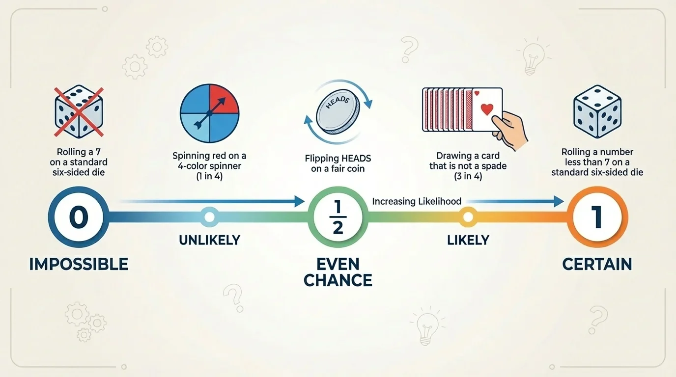
Events with probabilities close to \(0\) are unlikely. Events with probabilities close to \(1\) are likely. An event with probability around \(\dfrac{1}{2}\) is neither unlikely nor likely. It has about an even chance of happening.
This idea is important: larger probability numbers mean greater likelihood. An event with probability \(\dfrac{3}{4}\) is more likely than an event with probability \(\dfrac{1}{4}\). An event with probability \(0.9\) is more likely than one with probability \(0.2\).
Let us connect numbers to meaning:
Here are some examples:
| Probability | Meaning | Example |
|---|---|---|
| \(0\) | Impossible | Rolling a \(9\) on a standard number cube |
| \(0.1\) | Very unlikely | Choosing a particular student from a large school |
| \(\dfrac{1}{2}\) | Neither likely nor unlikely | Flipping heads on a fair coin |
| \(0.75\) | Likely | Choosing a vowel from the letters in "MATHA" |
| \(1\) | Certain | Picking a month that has at least \(28\) days |
Table 1. Probabilities and their meanings on the scale from \(0\) to \(1\).
Notice that probability is not just a number to calculate. It also tells a story about what to expect. If one event has probability \(0.8\) and another has probability \(0.3\), the first event is much more likely, even though neither result is guaranteed.
The probability scale as a measuring tool
Probability works like a measuring tool for uncertainty. Just as length is measured in units and temperature is measured in degrees, likelihood is measured with numbers from \(0\) to \(1\). The closer the value is to \(1\), the stronger the expectation that the event will happen. The closer it is to \(0\), the weaker that expectation becomes.
Another way to think about this is to compare probability to a dimmer switch instead of a simple on-off switch. It is not just "will happen" or "will not happen." Probability gives shades in between.
Probability can be written as a fraction, decimal, or percent. These forms mean the same thing when they represent the same value.
For example, the following all describe the same probability:
\(\dfrac{1}{2} = 0.5 = 50\%\)
Likewise, \(\dfrac{3}{4} = 0.75 = 75\%\). When a weather report says there is a \(75\%\) chance of rain, that means the probability of rain is \(0.75\), which is near \(1\), so rain is likely.
Fractions are often useful when we count outcomes. Decimals and percents are common in real life because they are easier to compare quickly.
Equivalent forms are important here. A fraction such as \(\dfrac{1}{4}\), a decimal such as \(0.25\), and a percent such as \(25\%\) can all describe the same probability.
Whatever form you use, the value must stay between \(0\) and \(1\), or between \(0\%\) and \(100\%\). A "probability" of \(1.4\) or \(140\%\) does not make sense for one event happening.
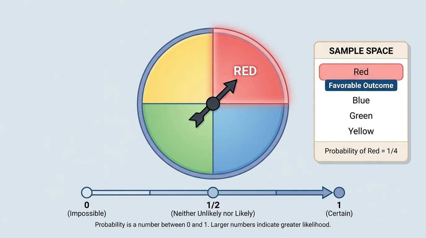
[Figure 2] Many beginning probability problems use equally likely outcomes. This means each possible outcome has the same chance of happening. A fair coin, a fair number cube, or a spinner with equal sections are common examples.
To find probability in these cases, we use this idea:
\[\textrm{Probability of an event} = \frac{\textrm{number of favorable outcomes}}{\textrm{total number of possible outcomes}}\]
The set of all possible outcomes is called the sample space. The outcomes that match the event are called favorable outcomes. In a spinner model, seeing all equal sections makes it easier to count both the total outcomes and the favorable ones.
Suppose a fair spinner has \(4\) equal sections: red, blue, green, and yellow. The total number of outcomes is \(4\). If the event is "landing on red," there is \(1\) favorable outcome. So the probability is \(\dfrac{1}{4}\).
If the event is "landing on a color that starts with the letter b," only blue works, so the probability is still \(\dfrac{1}{4}\). If the event is "landing on red or blue," then there are \(2\) favorable outcomes out of \(4\), so the probability is \(\dfrac{2}{4} = \dfrac{1}{2}\).
Notice how the value changes depending on how many favorable outcomes there are. More favorable outcomes mean a larger probability and a greater chance of the event happening.
Worked example 1
A fair coin is flipped once. What is the probability of landing on heads?
Step 1: List the possible outcomes.
The outcomes are heads and tails, so there are \(2\) possible outcomes.
Step 2: Count the favorable outcomes.
The event "heads" has \(1\) favorable outcome.
Step 3: Write the probability.
The probability is \(\dfrac{1}{2}\).
So the probability of landing on heads is \[\frac{1}{2}\]. This means heads is neither unlikely nor likely; it has an even chance.
A fair coin is one of the clearest examples of a situation with probability \(\dfrac{1}{2}\). That is why coin flips are often used to model equal chance.
Worked example 2
A standard number cube is rolled once. What is the probability of rolling a number greater than \(4\)?
Step 1: List the possible outcomes.
The sample space is \(\{1,2,3,4,5,6\}\), so there are \(6\) total outcomes.
Step 2: Identify the favorable outcomes.
Numbers greater than \(4\) are \(5\) and \(6\), so there are \(2\) favorable outcomes.
Step 3: Form the ratio.
The probability is \(\dfrac{2}{6}\).
Step 4: Simplify.
\(\dfrac{2}{6} = \dfrac{1}{3}\).
The probability of rolling a number greater than \(4\) is \[\frac{1}{3}\]. Since \(\dfrac{1}{3}\) is less than \(\dfrac{1}{2}\), the event is somewhat unlikely.
This example shows that a probability does not have to be extremely small to be unlikely. Any probability below \(\dfrac{1}{2}\) means the event happens less often than not.
Worked example 3
A bag contains \(5\) blue marbles, \(3\) green marbles, and \(2\) red marbles. One marble is chosen at random. What is the probability of choosing a green marble?
Step 1: Find the total number of marbles.
\(5 + 3 + 2 = 10\), so there are \(10\) marbles in all.
Step 2: Count the favorable outcomes.
There are \(3\) green marbles.
Step 3: Write the probability.
The probability is \(\dfrac{3}{10}\).
The probability of choosing a green marble is \[\frac{3}{10}\]. Since \(\dfrac{3}{10} = 0.3\), this event is unlikely, but not impossible.
Now compare that to choosing a blue marble. The probability would be \(\dfrac{5}{10} = \dfrac{1}{2}\), which is right at even chance. As we saw with the spinner in [Figure 2], counting favorable outcomes carefully is the key idea.
Worked example 4
A card is chosen from a set of cards numbered \(1\) through \(8\). What is the probability of choosing an even number?
Step 1: Identify the total outcomes.
There are \(8\) cards.
Step 2: Identify the favorable outcomes.
The even numbers are \(2, 4, 6, 8\), so there are \(4\) favorable outcomes.
Step 3: Calculate the probability.
\(\dfrac{4}{8} = \dfrac{1}{2}\).
The probability is \[\frac{1}{2}\]. This event is neither unlikely nor likely.
These examples show an important pattern: probability compares "how many ways the event can happen" to "how many outcomes are possible in all."
Because probability is a number, probabilities can be compared and ordered. If one event has a greater probability than another, it is more likely to happen.
For example, compare these probabilities:
Ordered from least likely to most likely, they are \(\dfrac{1}{5}, \dfrac{1}{2}, \dfrac{4}{5}\).
That means Event C is the most likely, Event A is the least likely, and Event B is in the middle. On the probability scale shown earlier in [Figure 1], Event A would be near \(0\), Event B would be in the middle, and Event C would be near \(1\).
| Event | Probability | Interpretation |
|---|---|---|
| A | \(\dfrac{1}{5}\) | Unlikely |
| B | \(\dfrac{1}{2}\) | Neither unlikely nor likely |
| C | \(\dfrac{4}{5}\) | Likely |
Table 2. Comparison of three probabilities and what each value means.
This is the heart of the topic: probability values do not just label events; they compare how strongly we expect events to occur.
Weather forecasts often use probability rather than yes-or-no predictions because the atmosphere is complex. A forecast with \(60\%\) chance of rain means rain is more likely than not, but dry weather is still possible.
That is why probability is so useful. It describes uncertainty in a precise way without pretending the future is perfectly known.
[Figure 3] Sometimes we know a probability from the structure of a situation, such as a fair coin or fair number cube. Other times, we estimate probability by repeating an experiment and recording results. This is called experimental probability. In repeated trials, real results can be compared with expected probabilities.
Experimental probability is found by using actual data:
\[\textrm{Experimental probability} = \frac{\textrm{number of times the event occurs}}{\textrm{total number of trials}}\]
Suppose a coin is flipped \(20\) times and lands on heads \(12\) times. Then the experimental probability of heads is \(\dfrac{12}{20} = 0.6\).
That result is not exactly \(\dfrac{1}{2}\), even though the theoretical probability for a fair coin is \(\dfrac{1}{2}\). This does not mean the coin must be unfair. In small numbers of trials, results can vary. Over many trials, experimental results often move closer to the theoretical probability.
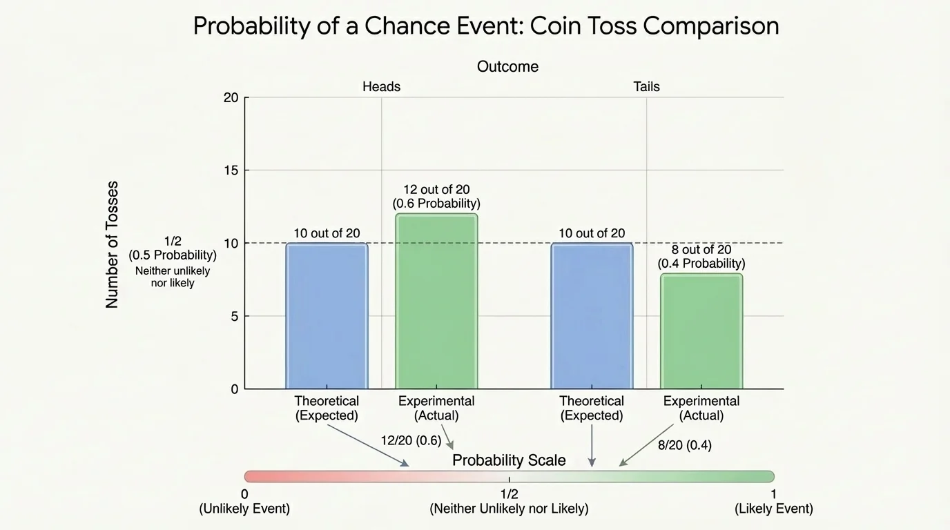
If the coin were flipped \(1,000\) times instead of \(20\) times, the experimental probability would often be closer to \(0.5\). This is one reason scientists and statisticians collect lots of data before drawing conclusions.
Experimental probability is especially useful when the exact theoretical model is hard to know in advance. In sports, for example, teams use past data to estimate the chance of a player making a shot. In medicine, researchers use data to estimate the likelihood of treatment success. The comparison in [Figure 3] reminds us that real results can differ from expected values, especially in short runs.
Probability is not just for games. It helps people make decisions in serious situations.
In weather forecasting, a \(90\%\) chance of snow means snow is very likely. That information helps schools, drivers, and city workers prepare. In sports, if a soccer player scores on \(80\%\) of penalty kicks, coaches know the player is very reliable, though missing is still possible.
In medicine, doctors may discuss the probability that a treatment will work or that a test result will be accurate. In engineering, designers consider the probability of system failure so they can build safer bridges, airplanes, and computers. In business, companies estimate the probability that customers will buy a product or that demand will rise.
All of these uses depend on one central idea: probability expresses likelihood using numbers from \(0\) to \(1\). Those numbers help people compare risks, benefits, and expectations.
"Probability is expectation written as a number."
— Mathematical idea behind chance models
That statement captures why probability matters. It turns uncertain situations into information people can reason about.
One common misunderstanding is thinking that a likely event is guaranteed. It is not. If the probability of rain is \(0.9\), rain is very likely, but a dry day can still happen.
Another misunderstanding is thinking an unlikely event can never happen. That is also false. If the probability is \(0.1\), the event is unlikely, not impossible. Unlikely events still occur sometimes.
A third misunderstanding comes from past results. Suppose a fair coin lands on tails \(5\) times in a row. Some people think heads is now "due." But if the coin is fair, the probability of heads on the next flip is still \(\dfrac{1}{2}\). Previous flips do not force the next result.
This is why probability must be interpreted carefully. It measures likelihood, not certainty, and it does not guarantee short-term patterns.
When you read or calculate a probability, ask these questions: What are all the possible outcomes? Which outcomes count for the event? Are the outcomes equally likely? Is the probability near \(0\), near \(\dfrac{1}{2}\), or near \(1\)?
These questions help you move from just calculating a number to understanding what the number means. That meaning is what makes probability powerful in statistics and in everyday decision-making.