Some rules describe change in a surprisingly simple way. If a streaming service charges a sign-up fee and then the same amount each month, or if a taxi charges a starting fee and then the same amount per mile, the total cost grows in a steady pattern. That kind of steady change is exactly what linear functions describe, and one of the most important ways to write them is with the equation \(y = mx + b\).
Linear relationships appear whenever one quantity changes by equal amounts as another quantity changes. If you walk at a constant speed, the distance you travel increases by the same amount each minute. If a job pays the same hourly rate, your earnings increase by the same amount each hour. These are not random patterns. They follow a rule.
A rule in algebra can define a function, which means each input has exactly one output. In a linear function, that rule creates a graph that is a straight line. That straight-line shape is not just a shape on paper. It tells us the change is steady and predictable.
You already know how to plot ordered pairs such as \((2,5)\), and you know that an equation can connect two variables. A function takes an input, often \(x\), and assigns exactly one output, often \(y\).
When we say a function is linear, we mean more than "it has an \(x\) in it." We mean that the function has a constant rate of change, and because of that constant rate, the graph forms a straight line.
A function matches each input value to one output value. If \(x\) is the input and \(y\) is the output, then a function rule tells you how to find \(y\) from \(x\). For example, in the rule \(y = 2x + 3\), if \(x = 4\), then \(y = 2(4) + 3 = 11\).
Functions can be shown in several ways: with an equation, a table, a graph, or a verbal description. In this topic, you compare functions in all of these forms to decide whether they are linear.
Linear function means a function with a constant rate of change. Its graph is a straight line.
Rate of change tells how much the output changes when the input changes.
Graph of a function is the set of points \((x,y)\) that satisfy the rule.
If the outputs increase or decrease by equal amounts when the inputs increase by equal amounts, the function is linear. If the amount of change keeps changing, the function is not linear.
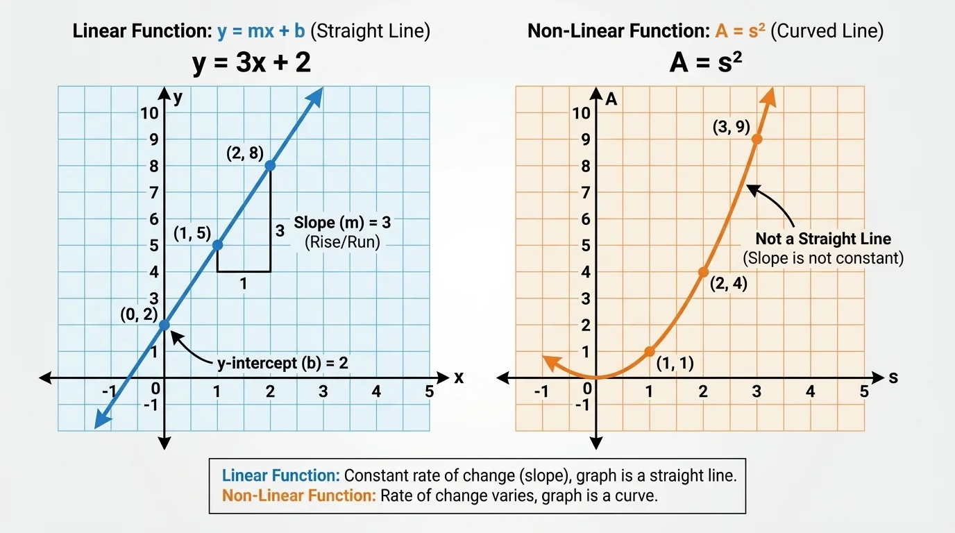
The equation \(y = mx + b\) is a special way to write a linear function. It gives two very important pieces of information about the line, as [Figure 1] shows: how steep the line is and where it crosses the \(y\)-axis.
In the equation \(y = mx + b\), the letter \(m\) is the slope. Slope tells the rate of change of the function. It tells how much \(y\) changes when \(x\) increases by \(1\). The letter \(b\) is the y-intercept. The \(y\)-intercept is the value of \(y\) when \(x = 0\), so it tells where the line crosses the \(y\)-axis.
For example, consider the equation \(y = 3x + 2\). Here, the slope is \(3\), so for every increase of \(1\) in \(x\), the value of \(y\) increases by \(3\). The \(y\)-intercept is \(2\), so the graph passes through the point \((0,2)\).
You can also think of \(y = mx + b\) as having two parts. The term \(mx\) controls how the output changes, and the term \(b\) gives the starting value. If \(b\) is positive, the line starts above the origin on the \(y\)-axis. If \(b\) is negative, it starts below the origin.
Slope can also be negative, zero, or a fraction. In \(y = -2x + 5\), the slope is \(-2\), so as \(x\) increases, \(y\) decreases by \(2\) each time. In \(y = \dfrac{1}{2}x + 1\), the slope is \(\dfrac{1}{2}\), so \(y\) increases by \(1\) when \(x\) increases by \(2\). In \(y = 4\), the slope is \(0\), so the graph is a horizontal line.
Why \(y = mx + b\) always graphs as a straight line
If the output changes at a constant rate, then equal horizontal moves on the graph create equal vertical moves. That repeated, steady pattern places the points in a straight path. The graph is straight because the relationship changes evenly, not because of a drawing trick.
As you continue, remember that a linear function does not have exponents on the variable other than \(1\), and the variable does not appear multiplied by itself. Forms like \(y = 2x + 7\) and \(y = -5x - 1\) are linear. Forms like \(y = x^2\) or \(y = \dfrac{1}{x}\) are not linear.
A graph helps you see linearity quickly. If the points lie on one straight line, the function is linear. If the graph bends or curves, the function is not linear.
The idea of a constant rate of change is the key. Suppose a table shows that when \(x\) goes from \(1\) to \(2\) to \(3\), the \(y\)-values go from \(4\) to \(7\) to \(10\). Each time \(x\) increases by \(1\), \(y\) increases by \(3\). That constant difference means the function is linear.
Now compare that to a table where \(x\) goes from \(1\) to \(2\) to \(3\), but \(y\) goes from \(1\) to \(4\) to \(9\). The changes in \(y\) are \(3\) and then \(5\), not equal. Since the rate of change is not constant, the function is not linear.
That difference is visible on a graph too. The line in [Figure 1] stays straight because the rate of change stays the same everywhere on the graph.
You can decide whether a function is linear by looking at its equation, table, or graph. A useful comparison appears in [Figure 2], where a straight-line graph and a curved graph show the difference clearly.
If an equation can be written in the form \(y = mx + b\), then it is linear. For example, \(y = 5x - 4\) is linear. The slope is \(5\), and the \(y\)-intercept is \(-4\).
But some functions are not linear. For example, the function \(A = s^2\) gives the area of a square as a function of its side length. This is not linear because the graph contains the points \((1,1)\), \((2,4)\), and \((3,9)\), and those points do not lie on a straight line.
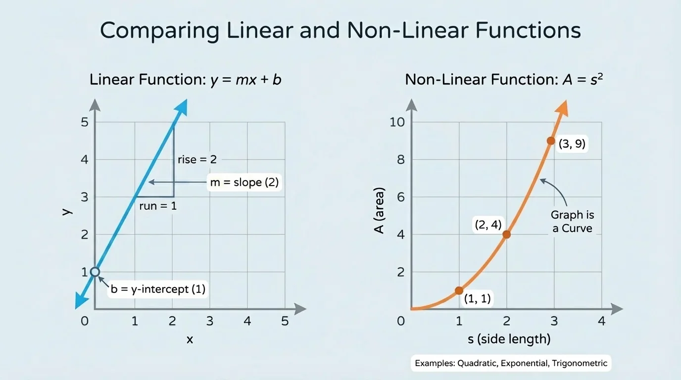
Notice what happens in the square-area function. If the side length increases from \(1\) to \(2\), the area increases from \(1\) to \(4\), which is an increase of \(3\). If the side length increases from \(2\) to \(3\), the area increases from \(4\) to \(9\), which is an increase of \(5\). The change is not constant, so the function is not linear.
Here are more examples.
| Function | Linear or Not? | Reason |
|---|---|---|
| \(y = 4x + 1\) | Linear | It is in the form \(y = mx + b\). |
| \(y = -3x\) | Linear | It is in the form \(y = mx + b\) with \(b = 0\). |
| \(y = x^2 + 2\) | Not linear | The variable has exponent \(2\). |
| \(y = \dfrac{2}{x}\) | Not linear | The rate of change is not constant. |
| \(A = s^2\) | Not linear | The graph is curved, not straight. |
Table 1. Comparison of linear and non-linear functions using equations and reasons.
A function can be increasing and still not be linear. The square-area function \(A = s^2\) always gets larger as \(s\) gets larger, but it does not increase at a constant rate.
Another common mistake is thinking that every graph passing through the origin is linear. That is false. Some non-linear graphs also pass through \((0,0)\). What matters is whether the graph is a straight line and whether the rate of change is constant.
Now let's apply these ideas carefully. Each example shows how to evaluate, interpret, or classify a function.
Worked example 1
Find the slope, \(y\)-intercept, and output when \(x = 4\) for the function \(y = 2x - 3\).
Step 1: Identify \(m\) and \(b\).
Compare \(y = 2x - 3\) to \(y = mx + b\). This gives \(m = 2\) and \(b = -3\).
Step 2: Interpret the values.
The slope is \(2\), so \(y\) increases by \(2\) for each increase of \(1\) in \(x\). The \(y\)-intercept is \(-3\), so the line crosses the \(y\)-axis at \((0,-3)\).
Step 3: Evaluate the function at \(x = 4\).
Substitute \(x = 4\): \(y = 2(4) - 3 = 8 - 3 = 5\).
The output is \(5\), so the point \((4,5)\) is on the graph.
This example shows that a linear equation gives both a rule and a graph. You can read the behavior from the equation before even plotting points.
Worked example 2
Decide whether the table represents a linear function.
| \(x\) | \(y\) |
|---|---|
| \(0\) | \(1\) |
| \(1\) | \(4\) |
| \(2\) | \(7\) |
| \(3\) | \(10\) |
Table 2. A table used to test whether a function has a constant rate of change.
Step 1: Look at how \(x\) changes.
Each time, \(x\) increases by \(1\).
Step 2: Look at how \(y\) changes.
The \(y\)-values change from \(1\) to \(4\) to \(7\) to \(10\). The differences are \(3\), \(3\), and \(3\).
Step 3: Decide whether the rate of change is constant.
Because the change in \(y\) is always \(3\) when the change in \(x\) is \(1\), the rate of change is constant.
The function is linear. Its slope is \(3\), and because \(y = 1\) when \(x = 0\), the equation is \(y = 3x + 1\).
Tables are especially useful when no equation is given. A quick check of first differences can reveal whether a pattern is linear.
Worked example 3
Decide whether \(A = s^2\) is linear.
Step 1: Test several input values.
If \(s = 1\), then \(A = 1^2 = 1\). If \(s = 2\), then \(A = 2^2 = 4\). If \(s = 3\), then \(A = 3^2 = 9\).
Step 2: Write the points.
The points are \((1,1)\), \((2,4)\), and \((3,9)\).
Step 3: Check for a constant rate of change.
From \((1,1)\) to \((2,4)\), the output changes by \(3\). From \((2,4)\) to \((3,9)\), the output changes by \(5\). These are not equal.
The function is not linear because its graph is not a straight line, as the curved graph in [Figure 2] confirms.
This is an important example because the rule seems simple, but not every simple rule is linear. The exponent on the variable changes the behavior.
Worked example 4
Compare the functions \(y = x + 4\) and \(y = x^2 + 4\).
Step 1: Look at the structure of each equation.
The equation \(y = x + 4\) matches the form \(y = mx + b\), with \(m = 1\) and \(b = 4\).
The equation \(y = x^2 + 4\) has \(x^2\), so it does not match the linear form.
Step 2: Compare outputs.
For \(x = 1, 2, 3\), the first function gives \(5, 6, 7\). The second gives \(5, 8, 13\).
Step 3: Compare the changes.
In the first function, the outputs increase by \(1\) each time. In the second, they increase by \(3\) and then \(5\).
The function \(y = x + 4\) is linear, but \(y = x^2 + 4\) is not.
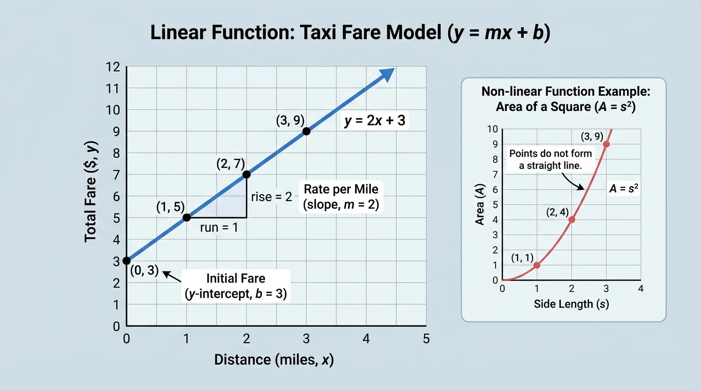
Linear functions are useful because many real situations involve a starting value plus a constant change. A taxi fare model often has a fixed starting fee and then the same charge for each mile.
[Figure 3] Suppose a taxi ride costs $3 to start and then $2 per mile. If \(x\) is the number of miles and \(y\) is the total cost, the equation is \(y = 2x + 3\). The slope is \(2\), which means the cost increases by $2 for each mile. The \(y\)-intercept is \(3\), which means the ride starts at $3 even before any miles are traveled.
Another example is earnings from a part-time job. If you earn $15 per hour, your pay \(P\) after \(h\) hours can be written as \(P = 15h\). This is a linear function with slope \(15\) and \(y\)-intercept \(0\). There is no starting amount, so the graph passes through the origin.
Temperature conversion also uses a linear function. The formula connecting Fahrenheit \(F\) and Celsius \(C\) is \(F = \dfrac{9}{5}C + 32\). The slope \(\dfrac{9}{5}\) tells how much Fahrenheit changes for each increase of \(1\) degree Celsius, and the intercept \(32\) tells the Fahrenheit value when \(C = 0\).
In each of these situations, the graph is a straight line because the change is constant. The steady pattern in the taxi graph in [Figure 3] is the same mathematical idea as the steady pattern in pay or temperature conversion.
Comparing linear functions
When two functions are both linear, you can compare them by their slopes and intercepts. A greater slope means a faster rate of change. A greater \(y\)-intercept means a larger starting value. For example, between \(y = 4x + 1\) and \(y = 2x + 5\), the first changes faster, but the second starts higher.
This kind of comparison matters in real decisions. One phone plan may have a low monthly fee but higher cost per gigabyte, while another may have a higher fee but lower usage cost. Linear functions help you compare those choices clearly.
One mistake is confusing a straight-looking list of numbers with a linear pattern. The values must change at a constant rate. If the differences are not equal, the function is not linear.
Another mistake is believing that any equation with variables is linear. For example, \(y = x^2 + 1\) is not linear, even though it looks simple. The exponent changes the rate of change, so the graph curves.
A third mistake is forgetting that \(b\) is the value when \(x = 0\). In \(y = 5x - 2\), the \(y\)-intercept is \(-2\), not \(2\). The line crosses the \(y\)-axis below the origin.
Finally, do not assume that all linear functions increase. If the slope is negative, the function is still linear, but the line goes downward from left to right. A straight line does not always mean a rising line.
"A straight line on a graph is the picture of constant change."
That idea connects equations, tables, graphs, and real situations. When you see a rule in the form \(y = mx + b\), you should immediately think of a constant rate of change, a straight-line graph, and the meaning of slope and intercept together.