A streaming service, a taxi ride, and a savings account can all follow the same mathematical idea: you start with some amount, and then the total changes by the same amount over and over. That pattern is powerful because once you recognize it, you can predict future values, compare situations, and write a rule that works every time. This kind of pattern is called a linear function.
Suppose a gym charges a $25 sign-up fee and then $10 each month. After one month, the cost is $35. After two months, it is $45. After three months, it is $55. The total keeps increasing by the same amount, which is \(10\) dollars per month. That constant change is the clue that the relationship is linear.
Linear functions help answer questions like these: How much will something cost after \(6\) months? How far will a bike travel in \(15\) minutes if the speed stays constant? How much water is left in a tank if the same amount drains each hour? In each case, one quantity depends on another in a steady way.
Linear relationship means two quantities change at a constant rate.
Rate of change is how much the output changes when the input changes by \(1\) unit.
Initial value is the starting amount, or the value of the function when the input is \(0\).
Function is a rule that gives exactly one output for each input.
A linear function is often written in the form
\(y = mx + b\)
In this equation, \(m\) is the rate of change and \(b\) is the initial value. If you know those two numbers, you know the whole function.
A linear relationship has a constant rate of change, and its graph is a straight line with the same steepness all the way across, as [Figure 1] shows. If the amount added or subtracted each step stays the same, the relationship is linear.
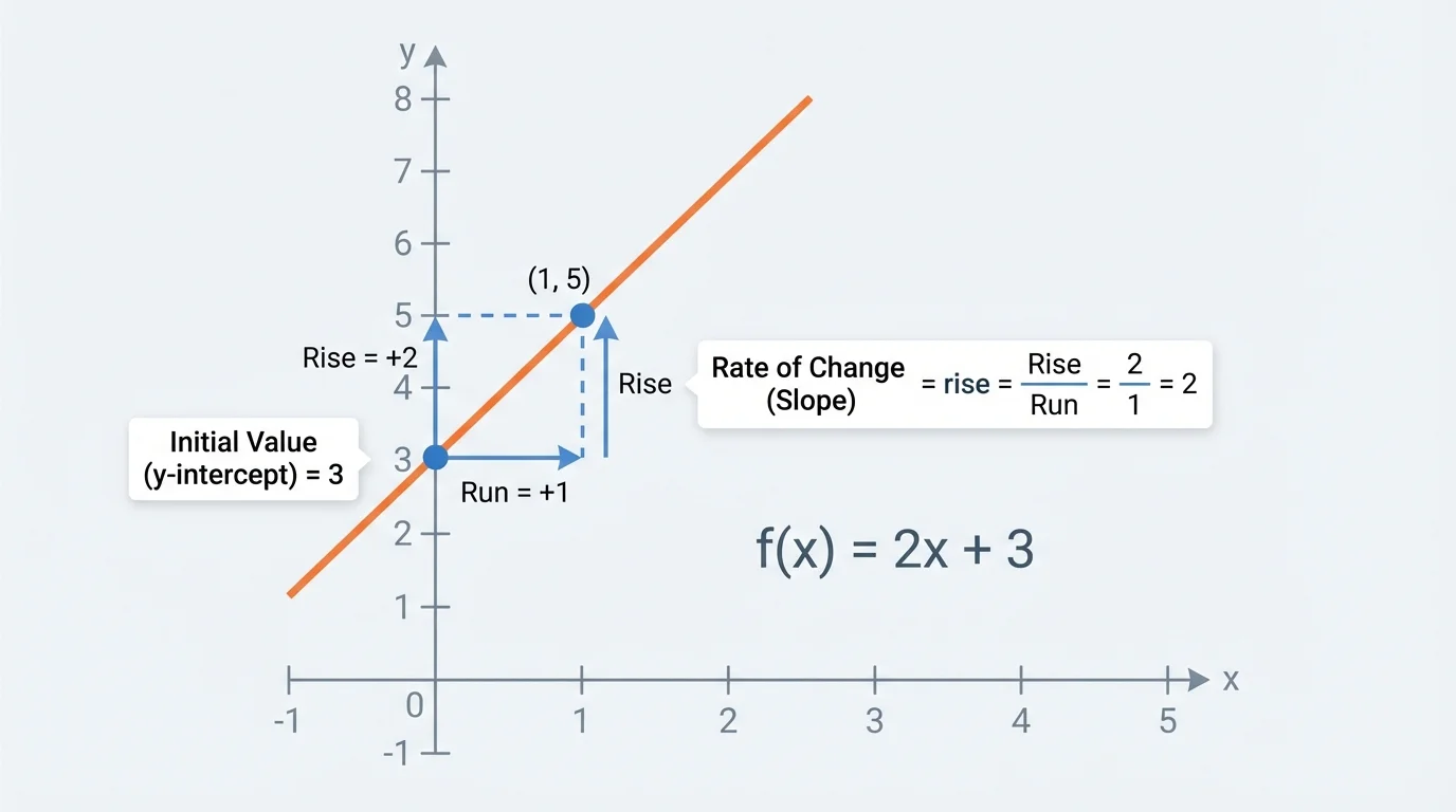
For example, in the function \(y = 2x + 3\), the output starts at \(3\) when \(x = 0\), and then it increases by \(2\) every time \(x\) increases by \(1\). If \(x\) goes from \(0\) to \(1\), \(y\) goes from \(3\) to \(5\). If \(x\) goes from \(1\) to \(2\), \(y\) goes from \(5\) to \(7\). The change is always \(+2\).
Not every pattern is linear. If the changes are \(+2\), then \(+4\), then \(+6\), the rate is not constant. That means the relationship is not linear.
On a graph, a positive rate of change means the line rises from left to right. A negative rate of change means the line falls from left to right. A rate of change of \(0\) means the line is horizontal.
The initial value is where the graph crosses the vertical axis, also called the y-intercept. In \(y = 2x + 3\), the graph crosses the \(y\)-axis at \(3\). That point is \((0,3)\).
The rate of change tells how fast one quantity changes compared with another. It can be positive, negative, or zero. For a linear function, the rate of change is also called the slope.
You can compute slope between two points \((x_1, y_1)\) and \((x_2, y_2)\) using
\[m = \frac{y_2 - y_1}{x_2 - x_1}\]
This formula compares the change in \(y\) to the change in \(x\). Another way to say that is rise over run.
The initial value is the value of \(y\) when \(x = 0\). In a context, it is the amount you start with before any change happens. In a graph, it is where the line crosses the \(y\)-axis. In a table, it is the output that matches input \(0\), if that row is shown.
When working with ordered pairs, the first number is the input \(x\), and the second number is the output \(y\). A point \((4,11)\) means when \(x = 4\), the function value is \(11\).
Units matter too. If a plant grows \(3\) centimeters each week, then the rate of change is \(3\) centimeters per week. If a tank loses \(5\) liters each minute, then the rate of change is \(-5\) liters per minute.
Many real situations directly tell you the initial value and the rate of change. When that happens, writing the function is straightforward: put the rate of change in place of \(m\), and put the initial value in place of \(b\).
Solved example 1
A bicycle rental shop charges an $8 fixed fee and $5 for each hour. Write a function for the total cost \(C\) after \(h\) hours.
Step 1: Identify the initial value.
The fixed fee is charged even before any riding happens, so the initial value is \(8\).
Step 2: Identify the rate of change.
The cost increases by \(5\) dollars for each hour, so the rate of change is \(5\).
Step 3: Write the function.
Using \(C = mh + b\), we get
\(C = 5h + 8\)
The model is \(C = 5h + 8\).
In this situation, \(5\) means the cost rises by $5 for every extra hour, and \(8\) means the starting charge before any hours are used.
Descriptions may also use words like starts with, initially, already has, or base fee. Those phrases often signal the initial value. Words like per hour, each mile, every week, or for each often signal the rate of change.
Sometimes you are not given the equation directly. Instead, you get two points and must build the function yourself. First find the slope. Then use one of the points to find the initial value.
Solved example 2
Find the linear function that passes through \((2,9)\) and \((5,15)\).
Step 1: Find the slope.
Use \(m = \dfrac{y_2-y_1}{x_2-x_1}\): \(m = \dfrac{15-9}{5-2} = \dfrac{6}{3} = 2\).
Step 2: Substitute into \(y = mx + b\).
Now the equation has the form \(y = 2x + b\).
Step 3: Use one point to find \(b\).
Substitute \((2,9)\): \(9 = 2(2) + b\). So \(9 = 4 + b\), which gives \(b = 5\).
Step 4: Write the function.
\(y = 2x + 5\)
The line has rate of change \(2\) and initial value \(5\).
You can check by substituting the other point: if \(x = 5\), then \(y = 2(5) + 5 = 15\), which matches. Checking is a great habit because it catches small mistakes quickly.
If the slope is negative, the same process still works. For instance, points \((1,12)\) and \((3,6)\) give slope \(m = \dfrac{6-12}{3-1} = \dfrac{-6}{2} = -3\). That means the function decreases by \(3\) units for every increase of \(1\) in \(x\).
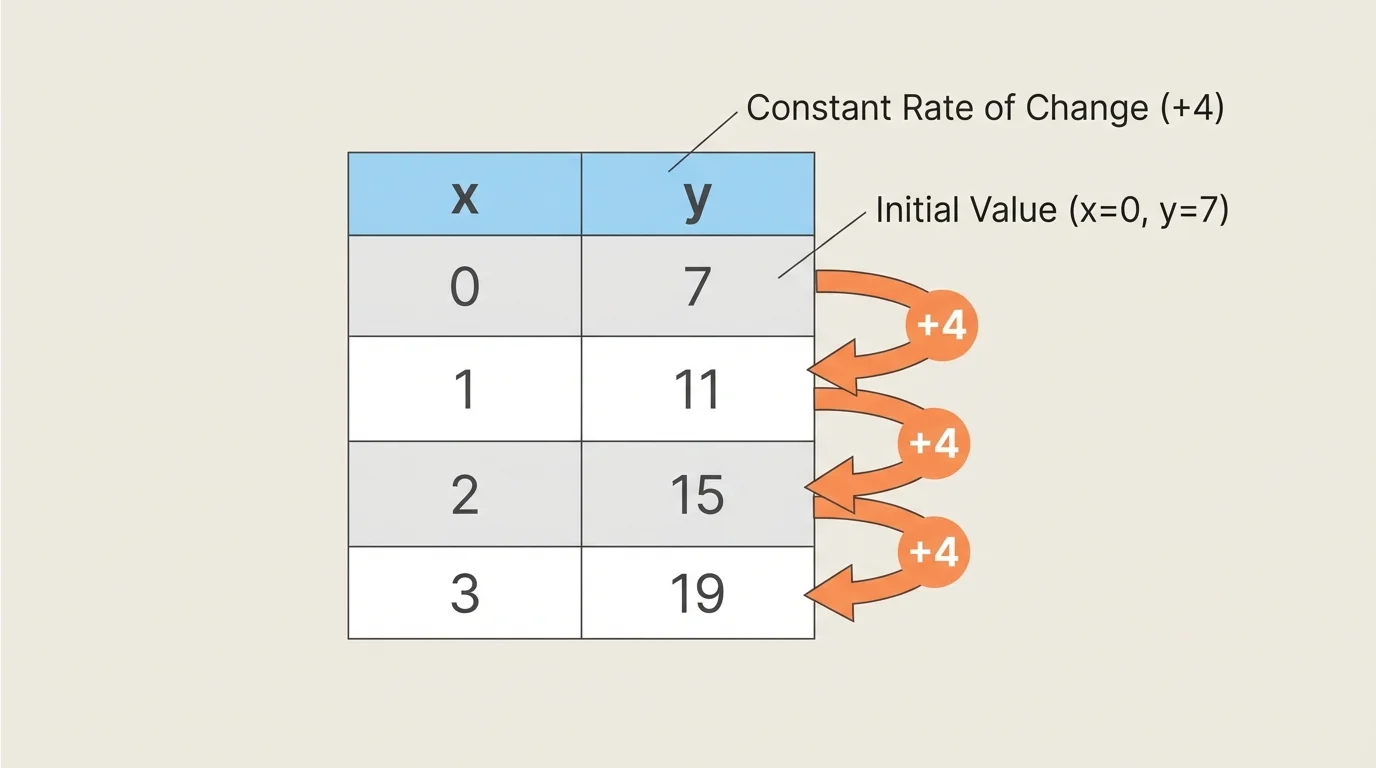
A table can reveal a linear pattern if the outputs change by a constant amount whenever the inputs increase by equal amounts. The pattern in [Figure 2] makes that visible because the differences between consecutive \(y\)-values stay the same.
If the \(x\)-values increase by \(1\), then you can find the rate of change just by looking at how much \(y\) changes each row. If the \(x\)-values increase by something other than \(1\), divide the change in \(y\) by the change in \(x\).
| \(x\) | \(y\) |
|---|---|
| \(0\) | \(7\) |
| \(1\) | \(11\) |
| \(2\) | \(15\) |
| \(3\) | \(19\) |
Table 1. A table in which the output increases by \(4\) each time the input increases by \(1\).
Here, the change in \(y\) is always \(+4\), so the rate of change is \(4\). Since the table includes \(x = 0\), we can read the initial value directly: when \(x = 0\), \(y = 7\). So the function is
\(y = 4x + 7\)
Solved example 3
Write a function for this table.
| \(x\) | \(y\) |
|---|---|
| \(2\) | \(14\) |
| \(4\) | \(20\) |
| \(6\) | \(26\) |
Table 2. A table where both inputs and outputs increase by constant amounts.
Step 1: Find the rate of change.
The input increases by \(2\), and the output increases by \(6\). So the rate of change is \(\dfrac{6}{2} = 3\).
Step 2: Use \(y = 3x + b\).
Substitute the point \((2,14)\): \(14 = 3(2) + b\).
Step 3: Solve for \(b\).
\(14 = 6 + b\), so \(b = 8\).
Step 4: Write the function.
\(y = 3x + 8\)
The function modeled by the table is \(y = 3x + 8\).
Later, when you compare tables and graphs, the constant difference pattern from [Figure 2] helps you quickly decide whether the data is linear.
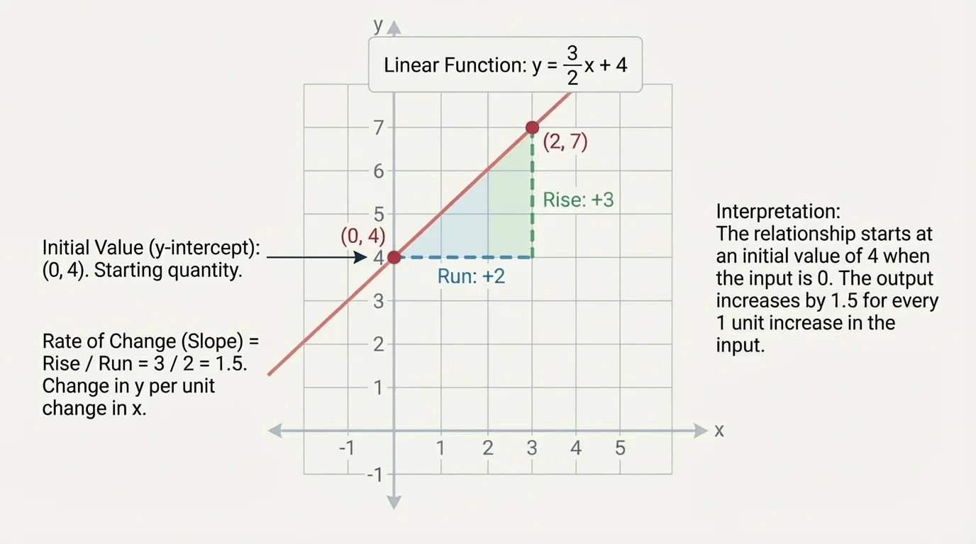
On a graph, slope can be seen as vertical change over horizontal change, and [Figure 3] shows this using a slope triangle between two points on the line. To read a linear function from a graph, first find the y-intercept, then pick two clear points to determine the rise and run.
Suppose a graph crosses the \(y\)-axis at \(4\), so the initial value is \(4\). Then choose two points, such as \((0,4)\) and \((2,10)\). The rise is \(10 - 4 = 6\), and the run is \(2 - 0 = 2\). So the slope is \(\dfrac{6}{2} = 3\). The function is \(y = 3x + 4\).
When reading from a graph, it is important to use points that lie exactly on grid intersections if possible. If the graph is drawn approximately, your answers may be estimates.
A graph also shows whether the function is increasing or decreasing. If the line rises, the function increases. If it falls, the function decreases. If it crosses the \(y\)-axis below \(0\), the initial value is negative.
As you move between a graph and an equation, keep matching parts: the slope tells the steepness, and the y-intercept tells where the line begins on the vertical axis. That same visual idea from [Figure 1] stays useful even when the numbers change.
Mathematics becomes more meaningful when the numbers are connected to a situation. In a real-world model, the rate of change and initial value must be interpreted using the units and the story.
Consider the function \(W = 120 - 8t\), where \(W\) is water in liters and \(t\) is time in minutes. The initial value is \(120\), meaning the tank starts with \(120\) liters. The rate of change is \(-8\), meaning the tank loses \(8\) liters each minute.
If a student writes the equation correctly but explains \(-8\) as the amount of water at the start, that interpretation is wrong. The number is correct, but the meaning is not. Understanding what each number represents is just as important as calculating it.
Numbers in a linear model always have jobs. The rate of change tells how one quantity changes compared with another. The initial value tells where the situation starts. In a graph, these appear as steepness and y-intercept. In a table, they appear as constant differences and the value at input \(0\), if shown.
A positive rate means growth, such as saving money each week. A negative rate means decrease, such as cooling temperature or fuel being used. A zero rate means the quantity stays constant.
One common mistake is mixing up the rate of change and the initial value. In \(y = 6x + 2\), the rate of change is \(6\), not \(2\). The initial value is \(2\), because that is the value when \(x = 0\).
Another mistake is forgetting to divide when the change in \(x\) is not \(1\). If \(y\) changes by \(10\) while \(x\) changes by \(5\), the rate of change is \(\dfrac{10}{5} = 2\), not \(10\).
A third mistake is assuming any set of points makes a line. To be linear, the slope between any two pairs of points must stay constant. If it does not, the relationship is not linear.
Small errors in reading a graph can change the equation a lot. That is why scientists and engineers often collect several data points and check whether the pattern is approximately linear before using a model to make predictions.
A useful check is substitution. If your function is supposed to fit a table or a pair of points, plug the input values into the equation and see whether the outputs match. If they do, your model is likely correct.
Linear functions appear everywhere because many situations change at an approximately constant rate over short periods of time.
A phone plan might cost $30 each month plus $0.05 for each text above a limit. A taxi fare might begin with a base charge and then increase by a certain amount per mile. A paycheck might be modeled by hourly rate times hours worked, sometimes with a starting bonus. In science, temperature can change at an almost constant rate during a short cooling process. In sports, distance often changes linearly with time when an athlete moves at steady speed.
Suppose a person already has $50 in savings and adds $12 each week. The model is \(S = 12w + 50\). Here, \(12\) means dollars per week, and \(50\) means the amount already saved. If someone else uses the model \(S = 10w + 70\), you can compare the two plans: one starts higher, but the other grows faster.
This is one reason linear models are useful: they help you compare situations, make predictions, and decide which choice is better for a certain goal.
"A pattern is not just something that repeats. It is something that can be described by a rule."
When you read descriptions, tables, graphs, and points as different views of the same function, the topic becomes much easier. A line on a graph, a constant difference in a table, and an equation like \(y = mx + b\) are all connected representations of one relationship.