A scientist grows plants under different amounts of sunlight and notices a pattern: plants that get more sunlight usually grow taller. A coach tracks practice time and sees that more practice often leads to better performance. A delivery company sees that longer distances usually mean longer travel times. These situations may look different, but they all involve a powerful idea in data analysis: two measurements can be related in a pattern, and a linear model can help describe that pattern and solve real problems.
When data involve two variables measured on the same object or person, they are called bivariate data. For example, a biology experiment might record hours of sunlight per day and mature plant height. A sports study might record hours of training and race time. Each pair of numbers belongs together because both measurements describe the same case.
If we graph bivariate data on a coordinate plane, we often use a scatter plot. Each point shows one pair of values. If the points seem to follow a straight-line pattern, a linear model may be a good way to describe the association. The model does not have to pass through every point exactly. Instead, it gives a line that represents the overall trend.
Association is a relationship between two variables. A linear model is an equation of a line used to describe an approximately straight-line pattern in bivariate data. The model helps predict the value of one variable from the value of the other.
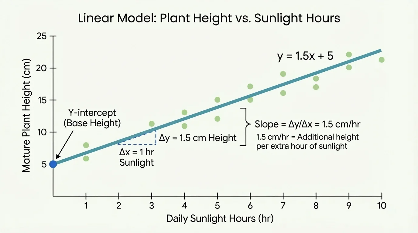
[Figure 1] A linear model is especially useful when the data show that as one variable changes, the other changes at a fairly steady rate. That steady rate is the heart of linear thinking.
A linear model is usually written in the form \(y = mx + b\). In this equation, \(x\) is the input variable, \(y\) is the predicted output variable, \(m\) is the slope, and \(b\) is the intercept. The slope tells how steep the line is, while the intercept tells where the line crosses the \(y\)-axis.
Suppose a biology experiment is modeled by \(h = 1.5s + 8\), where \(s\) is the number of sunlight hours per day and \(h\) is mature plant height in centimeters. This equation tells us two important things right away. First, the slope is \(1.5\), so each additional hour of sunlight is associated with an additional \(1.5\) centimeters of mature height. Second, the intercept is \(8\), so when \(s = 0\), the model predicts a mature height of \(8\) centimeters.
In real data, the phrase is associated with matters. A linear model describes a pattern in the data. It does not automatically prove that one variable causes the other. In some experiments, cause may be supported by careful design, but in many situations the model only describes how the variables move together.
You already know that points on a line can be described with coordinates \((x, y)\). You also know that substituting a value for \(x\) into an equation gives the corresponding value of \(y\). Linear models use that same idea, but now the variables represent real measurements.
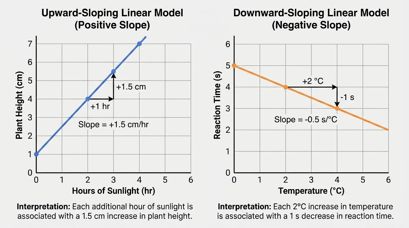
[Figure 2] The slope is one of the most important parts of a linear model because it tells the rate of change. In a model \(y = mx + b\), the slope is \(m\). A positive slope means the line rises from left to right, while a negative slope means the line falls from left to right.
To interpret slope correctly, always include the units. If the model is \(h = 1.5s + 8\), then the slope \(1.5\) means \(1.5\) centimeters per hour of sunlight. In words: an additional hour of sunlight each day is associated with an additional \(1.5\) centimeters of mature plant height.
Here are common ways slope can appear in context:
For example, if a runner's training model is \(t = -0.4h + 18\), where \(h\) is training hours per week and \(t\) is race time in minutes, the slope \(-0.4\) means each additional hour of training is associated with a decrease of \(0.4\) minutes in race time. That is about \(24\) seconds faster per extra hour, since \(0.4 \times 60 = 24\).
Why slope matters
Slope is not just a number attached to a line. It tells how much the predicted output changes for each increase of \(1\) unit in the input. In measurement data, this lets you explain the relationship in everyday language, not just symbol form.
The intercept is the predicted value of \(y\) when \(x = 0\). In the equation \(y = mx + b\), the intercept is \(b\). This is sometimes called the y-intercept because it is where the line crosses the \(y\)-axis on a graph.
For the model \(h = 1.5s + 8\), the intercept is \(8\). That means if a plant gets \(0\) hours of sunlight per day, the model predicts a mature height of \(8\) centimeters. Mathematically, this is easy to find: substitute \(s = 0\), and \(h = 1.5(0) + 8 = 8\).
But context matters. Sometimes the intercept makes sense, and sometimes it does not. If the experiment only measured plants receiving between \(4\) and \(10\) hours of sunlight, then \(0\) hours may be outside the observed data. The model still has an intercept, but that prediction may not be realistic. A line always crosses the \(y\)-axis somewhere; real life is not always that simple.
Once you have a linear model, you can use it to predict values by substituting a known input into the equation. This is one of the main reasons linear models are useful. They turn a trend in data into a tool for solving problems.
For example, if plant height is modeled by \(h = 1.5s + 8\), and a plant gets \(6\) hours of sunlight per day, then the predicted mature height is found by substitution: \(h = 1.5(6) + 8 = 9 + 8 = 17\). So the model predicts a mature height of \(17\) centimeters.
You can also work backward. If the model is \(h = 1.5s + 8\) and you want to know how many sunlight hours are associated with a mature height of \(20\) centimeters, set \(h = 20\) and solve:
\[20 = 1.5s + 8\]
Subtract \(8\): \(12 = 1.5s\). Then divide by \(1.5\): \(s = 8\). The model associates \(8\) hours of sunlight per day with a mature height of \(20\) centimeters.
Scientists, economists, coaches, and engineers all use linear models because they are simple enough to work with quickly but powerful enough to reveal patterns in real data.
Worked examples help show how the equation of a linear model answers different kinds of questions: predicting outputs, interpreting parameters, and solving for inputs.
Example 1: Predicting plant height
A biology experiment uses the model \(h = 1.5s + 8\), where \(s\) is sunlight hours per day and \(h\) is mature height in centimeters. Predict the mature height for a plant that gets \(7\) hours of sunlight each day.
Step 1: Identify the model and substitute the input value.
Replace \(s\) with \(7\): \(h = 1.5(7) + 8\).
Step 2: Multiply and add.
\(1.5 \times 7 = 10.5\), so \(h = 10.5 + 8 = 18.5\).
Step 3: Write the answer in context.
The predicted mature height is \(18.5\) centimeters.
This means the model predicts that a plant getting \(7\) hours of sunlight will reach a height of \(18.5\) cm.
Notice that this prediction comes from the model, not from measuring an actual plant. It is an estimate based on the pattern in the data.
Example 2: Interpreting a negative slope
A running coach models race time with \(t = -0.4h + 18\), where \(h\) is hours of training per week and \(t\) is race time in minutes.
Step 1: Identify the slope and intercept.
The slope is \(-0.4\), and the intercept is \(18\).
Step 2: Interpret the slope.
For each additional \(1\) hour of training per week, the predicted race time decreases by \(0.4\) minutes.
Step 3: Interpret the intercept.
When \(h = 0\), the model predicts a race time of \(18\) minutes.
So the model says more training is associated with faster race times, and someone with no weekly training is predicted to run the race in \(18\) minutes.
Negative slope does not mean something is wrong. It simply means the variables move in opposite directions. A downward line represents that kind of association.
Example 3: Solving for an input value
A taxi company models trip cost with \(C = 2d + 5\), where \(d\) is distance in miles and \(C\) is cost in dollars. How many miles does the model associate with a \(\$17\) trip?
Step 1: Substitute the known output.
Set \(C = 17\): \(17 = 2d + 5\).
Step 2: Solve the equation.
Subtract \(5\): \(12 = 2d\). Then divide by \(2\): \(d = 6\).
Step 3: State the result in context.
The model associates a \(\$17\) fare with a trip of \(6\) miles.
The slope \(2\) means the fare increases by \(\$2\) for each additional mile, and the intercept \(5\) represents the starting fee.
These examples show that the same equation can answer several different kinds of questions. You can interpret it, use it to predict, or solve it for a missing value.
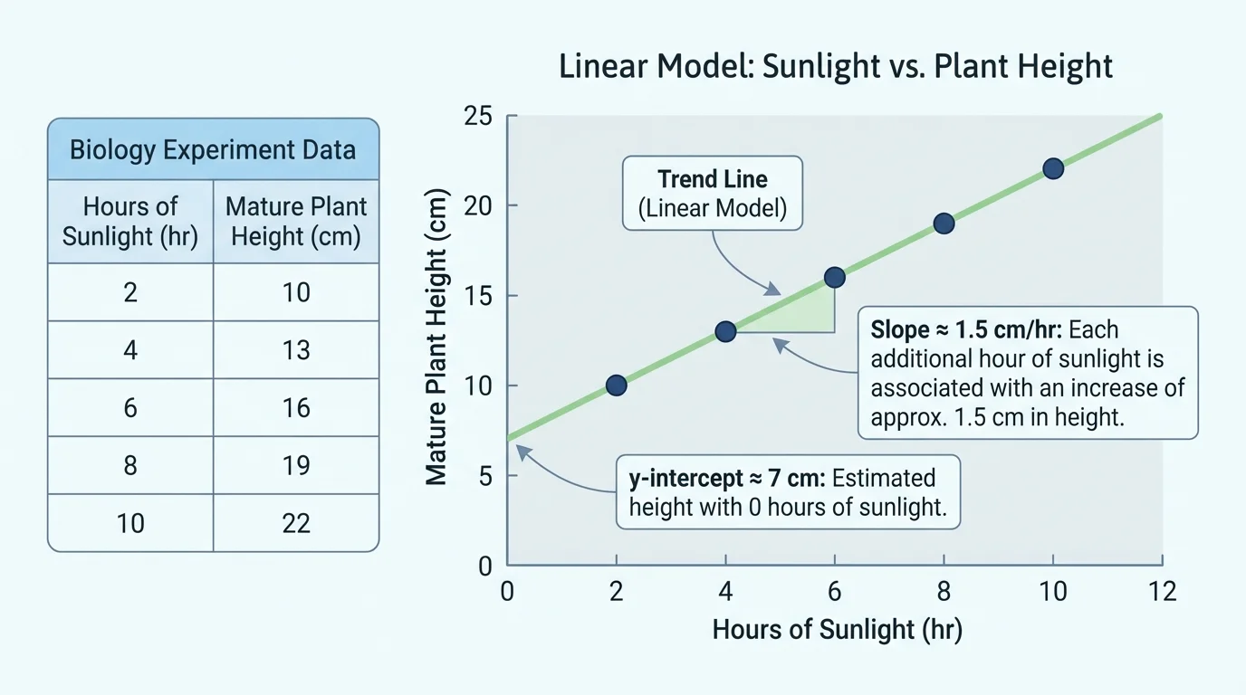
The same linear relationship can appear as a table, a graph, or an equation. Students become more proficient in statistics when they can move between all three forms. A data table and a scatter plot can represent the same association, while the equation gives a compact rule for predicting values.
Suppose study time \(x\) and quiz score \(y\) are modeled by \(y = 5x + 60\). If a table shows that more study time tends to go with higher scores, the graph should show points trending upward, and the equation should have a positive slope. All three representations should agree.
| Study time \((x)\) | Predicted quiz score \((y)\) |
|---|---|
| \(0\) | \(60\) |
| \(1\) | \(65\) |
| \(2\) | \(70\) |
| \(3\) | \(75\) |
Table 1. Predicted quiz scores from the linear model \(y = 5x + 60\).
From the table, every increase of \(1\) hour in study time increases the predicted score by \(5\) points. That increase of \(5\) is the slope. The score of \(60\) when \(x = 0\) is the intercept. Looking at a table this way helps you recognize slope and intercept even before writing the equation.
Later, when you compare data and models, it helps to remember that a line is not separate from the data. The model is built to describe the pattern in the points.
Linear models are useful, but they are not magic. A model is an approximation. Real data may be noisy, and not every relationship stays linear forever.
One important idea is interpolation, which means making a prediction within the range of the data. If your sunlight data run from \(4\) to \(10\) hours, predicting for \(6\) hours is interpolation. This is usually more reliable.
Another important idea is extrapolation, which means making a prediction outside the range of the data. If the same experiment only measured \(4\) to \(10\) hours of sunlight, predicting for \(20\) hours is extrapolation. That can be risky because the pattern may not continue in the same way.
Reasonable interpretation matters
Even if an equation is mathematically correct, its interpretation must fit the real situation. A negative predicted height, a quiz score above \(100\), or a travel time below \(0\) would signal that the model is being used outside a sensible range.
Linear models appear in many fields because they help people understand measurement data quickly. In science, a model can connect temperature and dissolved oxygen, fertilizer amount and plant growth, or time and distance. In medicine, a model can describe how dosage changes with body mass in a simplified study. In sports, coaches use linear trends to compare training time and performance. In business, companies may model shipping cost or fuel use.
Here are several context-based interpretations:
In each case, the equation is not just a rule for calculation. It tells a story about how two measured quantities are related.
"A good model does not capture every detail. It highlights the pattern that matters."
When you read or write a linear model, ask two questions every time: What does the slope mean in this situation, and what does the intercept mean in this situation? Those two ideas unlock almost everything important about the equation.