A modern city runs on hidden grids of information: bus routes, phone connections, sports schedules, online recommendations, and business profits can all be organized in rectangular arrays of numbers. Those arrays are called matrices, and they let us do something powerful: represent complicated systems clearly and then use operations to extract useful results. What looks like a simple table can actually become a mathematical tool for predicting revenue, comparing strategies, or describing a network of connections.
A matrix is useful whenever data naturally falls into rows and columns. A school might track how many tickets are sold for different events in different seating sections. A company might compare profits under several pricing and advertising choices. A transportation system might record which stations are connected by which routes. In each case, the layout matters just as much as the numbers.
Unlike an ordinary list of values, a matrix keeps relationships organized. Each number sits in a specific position, and that position tells you what the number means. Because of this structure, matrices are not only for storing data; they are also for manipulating data in ways that match real situations.
You already know how to work with ordered pairs, tables, and arrays. A matrix extends those ideas: instead of just one row or one column, it can contain many rows and many columns, and each entry is identified by its row number and column number.
In high school mathematics, one important goal is learning when matrix operations make sense and what they mean. If you add two matrices, you are combining matching pieces of information. If you multiply a matrix by a number, you are scaling every entry. If you multiply two matrices, you are combining one set of relationships with another set in a structured way.
A matrix is a rectangular arrangement of numbers. If a matrix has \(m\) rows and \(n\) columns, its dimension is \(m \times n\). The number in row \(i\), column \(j\) is called an entry. The meaning of any entry comes from the row label and the column label together.
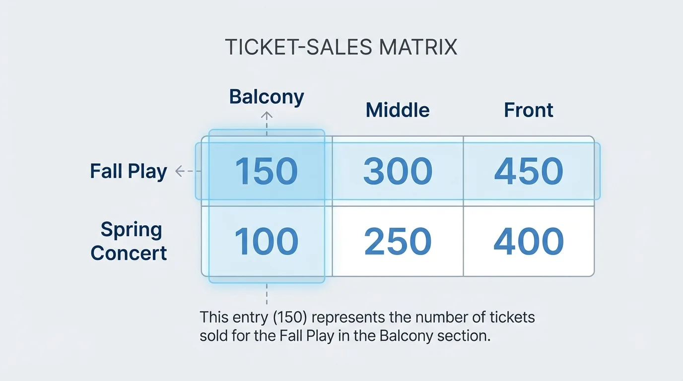
As [Figure 1] shows, suppose rows represent school events and columns represent seating sections. Then the matrix
\[A = \begin{bmatrix} 120 & 80 & 40\\150 & 90 & 60\end{bmatrix}\]
could mean that the first row is the fall play and the second row is the spring concert, while the columns are balcony, middle, and front seating. Then \(120\) is not just a number. It means \(120\) balcony tickets for the fall play.
Rows run horizontally, and columns run vertically. The dimension of a matrix tells its size, such as \(2 \times 3\). An entry is one number in a particular row and column position.
Context matters. The same matrix of numbers could represent tickets, survey results, or inventory counts. Mathematics gives the structure, but the real-world situation gives the interpretation.
Matrix notation helps us write data compactly. Instead of repeating full labels every time, we can refer to entry \(a_{ij}\), which means the number in row \(i\), column \(j\) of matrix \(A\). This notation becomes especially useful for larger data sets.
Many tables from everyday life can be turned directly into matrices. Suppose a snack stand records the number of sandwiches, fruit cups, and drinks sold on three days:
\[S = \begin{bmatrix} 35 & 20 & 50\\40 & 18 & 55\\30 & 25 & 48\end{bmatrix}\]
If the rows stand for Monday, Tuesday, and Wednesday, and the columns stand for sandwiches, fruit cups, and drinks, then each row gives one day's sales pattern, and each column tracks one product across several days.
Matrices are especially useful because they preserve this two-way organization. A list such as \(35, 20, 50, 40, 18, 55, ...\) loses the structure. The matrix keeps the categories visible.
Spreadsheets, computer graphics, recommendation systems, and parts of artificial intelligence all rely heavily on matrices. The same mathematics that organizes a school event table also helps streaming platforms connect users with movies they may enjoy.
When data comes from real situations, always ask two questions: what do the rows represent, and what do the columns represent? If you can answer both clearly, then you can interpret each matrix entry correctly.
Once data is placed into matrices, we can operate on it. But matrix operations are not allowed at random. The size of the matrices matters.
Two matrices are equal only if they have the same dimensions and the same corresponding entries. For matrix addition and subtraction, the matrices must also have the same dimensions. We add or subtract matching entries.
Solved example 1: Adding matrices
A theater records ticket sales on two weekends using the matrices
\[A = \begin{bmatrix}120 & 80\\ 100 & 60\end{bmatrix}, \qquad B = \begin{bmatrix}30 & 20\\ 25 & 15\end{bmatrix}\]
Find \(A + B\).
Step 1: Check the dimensions.
Both matrices are \(2 \times 2\), so addition is defined.
Step 2: Add corresponding entries.
\(120 + 30 = 150\), \(80 + 20 = 100\), \(100 + 25 = 125\), and \(60 + 15 = 75\).
Step 3: Write the result in matrix form.
\[A + B = \begin{bmatrix}150 & 100\\ 125 & 75\end{bmatrix}\]
This result represents total ticket sales across both weekends.
Scalar multiplication means multiplying every entry in a matrix by the same number. If a factory doubles production, the production matrix is multiplied by \(2\). If a survey sample is scaled down by half for estimation, the matrix may be multiplied by \(\dfrac{1}{2}\).
Solved example 2: Scalar multiplication
A cafeteria orders food quantities represented by
\[C = \begin{bmatrix}12 & 8 & 5\\ 10 & 6 & 4\end{bmatrix}\]
If an event expects three times as many guests, find \(3C\).
Step 1: Multiply each entry by \(3\).
\(3 \cdot 12 = 36\), \(3 \cdot 8 = 24\), \(3 \cdot 5 = 15\), \(3 \cdot 10 = 30\), \(3 \cdot 6 = 18\), and \(3 \cdot 4 = 12\).
Step 2: Write the new matrix.
\[3C = \begin{bmatrix}36 & 24 & 15\\ 30 & 18 & 12\end{bmatrix}\]
The scaled matrix shows the adjusted order amounts.
These operations are useful because they match real decisions. Addition combines data from similar categories. Subtraction compares changes. Scalar multiplication adjusts the size of every value in the same proportion.
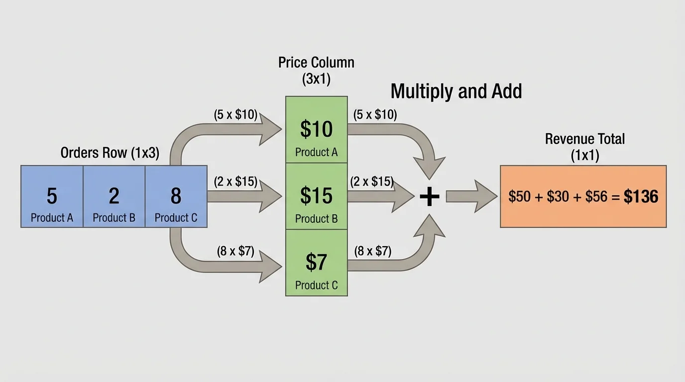
Matrix multiplication is more powerful than addition because it combines one set of data with another. As [Figure 2] illustrates, one row of one matrix can interact with one column of another matrix to produce a meaningful total.
If matrix \(A\) has size \(m \times n\) and matrix \(B\) has size \(n \times p\), then the product \(AB\) is defined and has size \(m \times p\). The inside dimensions must match. This is one of the most important checks in matrix work.
To find one entry of the product, multiply matching entries from a row of the first matrix and a column of the second matrix, then add the results. This is called the row-by-column rule.
Why matrix multiplication matters
[Figure 2] Suppose one matrix records how many items of each type were sold, and another matrix records the price of each item. Multiplying them can produce total revenue. Instead of doing many separate calculations by hand, matrix multiplication carries out the whole structure at once.
For example, let
\[O = \begin{bmatrix} 10 & 5 & 8\\7 & 12 & 6\end{bmatrix}\]
represent orders from two stores for three products, and let
\[P = \begin{bmatrix} 2\\ 3\\ 4\end{bmatrix}\]
represent prices in dollars for the three products. Then \(O\) is \(2 \times 3\) and \(P\) is \(3 \times 1\), so the product \(OP\) is defined and will be \(2 \times 1\).
Solved example 3: Matrix multiplication
Use
\[O = \begin{bmatrix}10 & 5 & 8\\ 7 & 12 & 6\end{bmatrix}, \qquad P = \begin{bmatrix}2\\3\\4\end{bmatrix}\]
to find \(OP\).
Step 1: Check dimensions.
\(O\) is \(2 \times 3\) and \(P\) is \(3 \times 1\). Since the inner dimensions \(3\) and \(3\) match, multiplication is defined.
Step 2: Compute the first entry.
Use row \(1\) of \(O\) and column \(1\) of \(P\): \(10 \cdot 2 + 5 \cdot 3 + 8 \cdot 4 = 20 + 15 + 32 = 67\).
Step 3: Compute the second entry.
Use row \(2\) of \(O\) and column \(1\) of \(P\): \(7 \cdot 2 + 12 \cdot 3 + 6 \cdot 4 = 14 + 36 + 24 = 74\).
Step 4: Write the product.
\[OP = \begin{bmatrix}67\\74\end{bmatrix}\]
The product gives total revenue for each store: $67 for the first store and $74 for the second.
This kind of calculation appears everywhere: nutrition totals from food quantities and nutrient values, total cost from item counts and prices, or total travel time from route segments and time per segment. The picture in [Figure 2] helps show why the process is not random; it links one kind of data to another kind.
One especially interesting application is the payoff matrix. A payoff matrix represents the outcome for different choices made by players, companies, or decision-makers. Rows may represent one player's strategies, and columns may represent another player's strategies.
Suppose a business must choose between two advertising plans, and a competitor must choose between two pricing plans. The resulting profits, in thousands of dollars, may be represented by
\[M = \begin{bmatrix} 12 & 6\\9 & 15\end{bmatrix}\]
If row \(1\) is online advertising, row \(2\) is mixed advertising, column \(1\) is high competitor pricing, and column \(2\) is low competitor pricing, then each entry shows the company's payoff in that situation.
Payoff matrices do not automatically tell us the "best" choice in every sense, because the answer depends on what the other side does. But they organize the possibilities clearly. Students often see this idea in game theory, economics, and strategy analysis.
Solved example 4: Interpreting a payoff matrix
Use
\[M = \begin{bmatrix}12 & 6\\ 9 & 15\end{bmatrix}\]
Answer these questions.
Step 1: Interpret entry \(m_{12}\).
Entry \(m_{12} = 6\) means the payoff is \(6\) thousand dollars when the company chooses online advertising and the competitor chooses low pricing.
Step 2: Find the larger payoff in column \(1\).
Column \(1\) contains \(12\) and \(9\). Since \(12 > 9\), online advertising gives the higher payoff if the competitor uses high pricing.
Step 3: Find the larger payoff in column \(2\).
Column \(2\) contains \(6\) and \(15\). Since \(15 > 6\), mixed advertising gives the higher payoff if the competitor uses low pricing.
The matrix shows that the stronger strategy depends on the competitor's action.
In some settings, payoff matrices contain gains and losses, so negative entries can appear. A negative value might mean a loss of money or a penalty in a game.
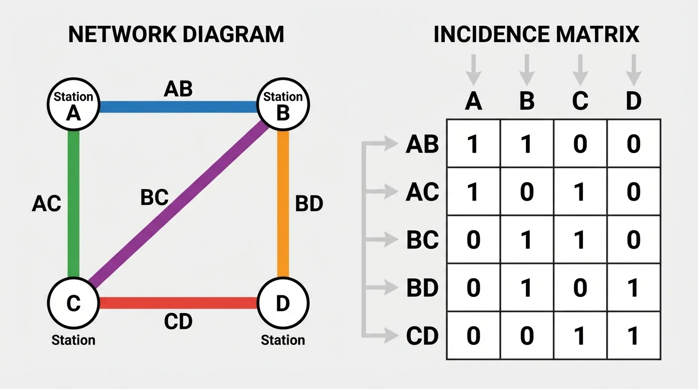
A network is a set of vertices connected by links. In mathematics, the links are often called edges. As [Figure 3] shows, a network can be translated into a matrix so that connections can be studied numerically.
An incidence matrix records which vertices and edges are connected. Usually, rows represent vertices and columns represent edges. An entry is often \(1\) if a vertex lies on an edge and \(0\) if it does not.
Consider a network with four stations: \(A\), \(B\), \(C\), and \(D\). Suppose the routes are \(e_1 = AB\), \(e_2 = AC\), \(e_3 = BC\), \(e_4 = BD\), and \(e_5 = CD\). Then an incidence matrix can be written as
\[I = \begin{bmatrix} 1 & 1 & 0 & 0 & 0\\1 & 0 & 1 & 1 & 0\\0 & 1 & 1 & 0 & 1\\0 & 0 & 0 & 1 & 1\end{bmatrix}\]
Here the rows correspond to \(A\), \(B\), \(C\), \(D\), and the columns correspond to \(e_1, e_2, e_3, e_4, e_5\). For example, column \(e_4\) has \(1\)s in rows \(B\) and \(D\), showing that route \(e_4\) connects \(B\) and \(D\).
Incidence matrices are useful because they turn a visual network into data that can be searched, counted, and manipulated. Engineers, computer scientists, and transportation planners all use related ideas when analyzing networks.
"Mathematics is the art of giving the same name to different things."
— Henri Poincaré
That quote fits matrices well: a theater schedule, a business strategy table, and a transit network may look different on the surface, but matrix structure lets us study them with a shared mathematical language.
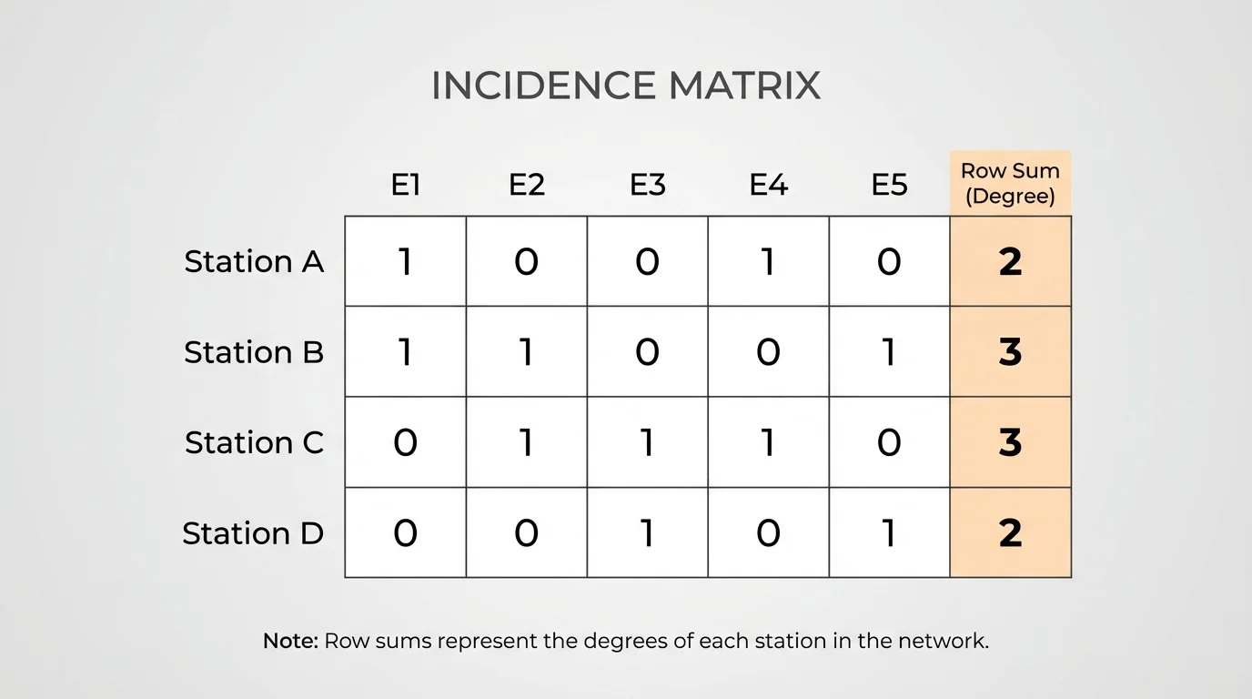
Matrices do more than store information. They often reveal patterns immediately. In network data, for example, row sums in an incidence matrix tell how many edges meet each vertex.
Using the matrix \(I\) above, the row sums are:
\(A: 1 + 1 + 0 + 0 + 0 = 2\), \(B: 1 + 0 + 1 + 1 + 0 = 3\), \(C: 0 + 1 + 1 + 0 + 1 = 3\), and \(D: 0 + 0 + 0 + 1 + 1 = 2\).
[Figure 4] That means stations \(B\) and \(C\) each connect to three routes, while \(A\) and \(D\) each connect to two. This is the kind of pattern transportation planners might notice when deciding which stations are the most connected.
In payoff matrices, patterns can reveal whether one strategy is often stronger than another. In sales matrices, row totals can give total sales for a day, while column totals can show the popularity of a product. In many applications, a zero entry is also meaningful: it may indicate no tickets sold, no connection, or no payoff.
Sometimes symmetry matters too. If a matrix representing mutual relationships is symmetric, then the entry in row \(i\), column \(j\) matches the entry in row \(j\), column \(i\). Although not every application produces a symmetric matrix, noticing this feature can simplify analysis.
The network view from [Figure 3] and the row-sum view from [Figure 4] show how visual structure and numerical structure work together. A matrix lets you move back and forth between the picture of a system and the calculations behind it.
One common mistake is trying to add or subtract matrices of different sizes. If one matrix is \(2 \times 3\) and another is \(3 \times 2\), addition is not defined because the entries do not match position by position.
Another common mistake is ignoring dimensions in multiplication. For \(AB\), the number of columns in \(A\) must equal the number of rows in \(B\). If not, the product does not exist. Even when multiplication is possible, \(AB\) and \(BA\) may have different sizes or one may exist while the other does not.
Meaning check
After every matrix operation, ask whether the result makes sense in context. If a product is supposed to represent total cost, its size should match the number of groups being priced. If an entry should count people or routes, a negative value would probably signal an error.
A good habit is to label rows and columns before calculating. This prevents a lot of confusion and helps you explain the result clearly.
Matrices are everywhere in modern life. In economics, payoff matrices help compare strategies under uncertainty. In transportation, incidence matrices describe how roads, routes, or rail lines connect locations. In sports, matrices can track wins, losses, or which teams play each other. In computer science, matrices help model networks, search engines, and communication links.
In manufacturing, one matrix may describe the number of parts needed for each product, while another lists the cost of each part. Multiplying them can give production costs. In school scheduling, a matrix can show which classrooms are used in which periods. In social networks, matrices can represent who is connected to whom.
| Application | Rows might represent | Columns might represent | Meaning of entries |
|---|---|---|---|
| Ticket sales | Events | Seating sections | Tickets sold |
| Payoff analysis | One player's strategies | Another player's strategies | Profit, score, or loss |
| Network incidence | Vertices or stations | Edges or routes | Whether a connection exists |
| Production and pricing | Stores or orders | Products | Quantities sold |
Table 1. Examples of how matrix rows, columns, and entries represent different types of real-world data.
What makes matrices so valuable is that one mathematical idea can handle many kinds of information. Whether the data describes money, movement, or connection, matrices provide a clean structure for both representation and calculation.