A graph is not just a picture. In algebra, it is a visual representation of all the solutions to an equation. Every point on the graph stands for an ordered pair that makes an equation true, and every point that does not fit the equation is left out. That idea is powerful because it turns algebra into something visible: a relationship such as \(y = 2x + 1\) becomes a whole set of points spread across the coordinate plane, and those points line up in a predictable shape.
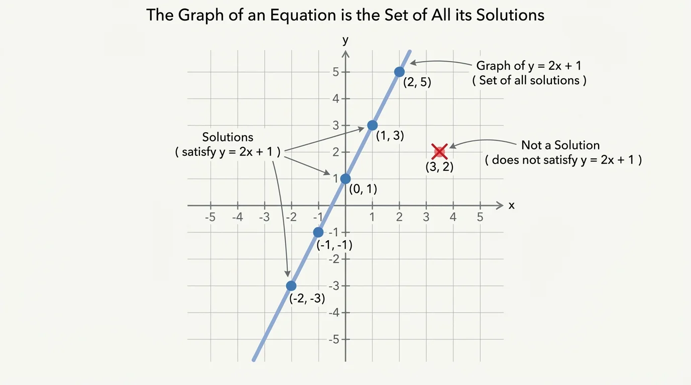
[Figure 1] An equation in two variables, such as \(x + y = 5\) or \(y = x^2\), usually has more than one solution. In fact, it often has infinitely many solutions. Each solution is an ordered pair \((x, y)\) that makes the equation true when the values are substituted.
For example, consider \(x + y = 5\). If \(x = 1\), then \(y = 4\), so \((1,4)\) is a solution. If \(x = 3\), then \(y = 2\), so \((3,2)\) is also a solution. If \(x = 5\), then \(y = 0\), so \((5,0)\) works too. When all such solution points are plotted on the coordinate plane, they form the graph of the equation.
Graph of an equation in two variables means the set of all points \((x,y)\) in the coordinate plane that make the equation true.
Solution means any ordered pair that satisfies the equation when substituted.
This is why the graph is not chosen randomly. It is built from the solutions. If a point is on the graph, the equation is true for that point. If a point is not on the graph, the equation is false for that point. Algebra and geometry are saying the same thing in two different languages.
The coordinate plane gives each ordered pair a location. The first number, \(x\), tells the horizontal position, and the second number, \(y\), tells the vertical position. Plot enough solution points, and a shape appears. Sometimes that shape is a straight line. Sometimes it bends into a curve. Either way, the graph is the complete collection of solutions, not just a few sample points.
Suppose you see a point on a graph at \((2,3)\). To say that point is a solution means that plugging \(x = 2\) and \(y = 3\) into the equation makes a true statement. For \(x + y = 5\), substitution gives \(2 + 3 = 5\), which is true, so \((2,3)\) belongs on the graph.
Now test \((2,4)\). Substituting gives \(2 + 4 = 6\), not \(5\). Since the equation is false, \((2,4)\) is not a solution and should not be on the graph. This simple check explains what a graph means at the most basic level.
From earlier work, you already know how to substitute values into an equation. That skill is essential here: graphical meaning depends on whether substitution makes the equation true or false.
This leads to an important interpretation rule: points on the graph satisfy the equation; points off the graph do not. That rule works for lines, parabolas, circles, and other curves. It also works whether the equation is written in standard form, slope-intercept form, or some other form.
Looking back to [Figure 1], the off-line point matters just as much as the points on the line. It reminds us that a graph is selective. The coordinate plane contains infinitely many points, but only the ones that satisfy the equation become part of its graph.
[Figure 2] Many students first meet graphing through linear equations, so it is easy to think every equation makes a line. But equations in two variables can produce many shapes.
A linear equation is an equation whose graph is a line. For example, \(y = 2x + 1\) gives a straight line because the rate of change is constant. Every time \(x\) increases by \(1\), \(y\) increases by \(2\). Some equations produce straight lines, while others produce curves.
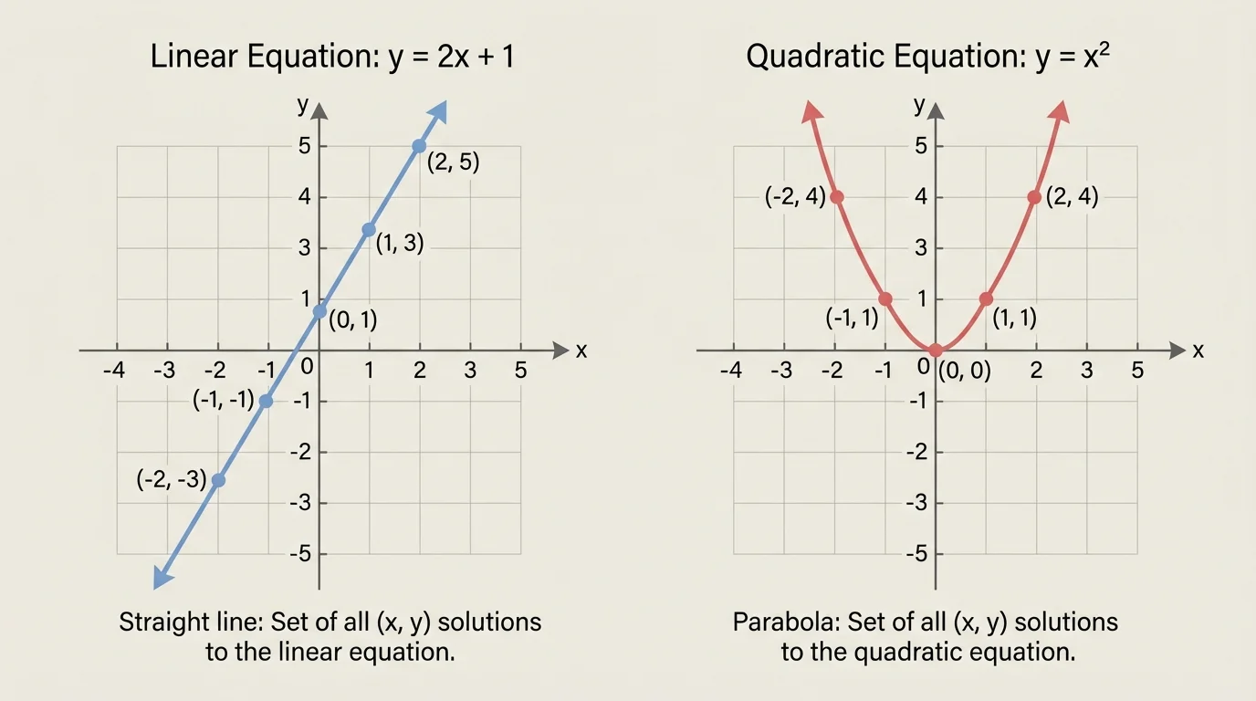
A curve is a graph that is not necessarily straight. For example, \(y = x^2\) forms a U-shaped graph called a parabola. The change in \(y\) is not constant, so the graph bends. Another example is \(x^2 + y^2 = 9\), which forms a circle centered at the origin with radius \(3\).
Shape comes from the relationship
The form of an equation determines the pattern of its solutions. A linear equation such as \(y = mx + b\) produces a line, while equations involving powers such as \(x^2\) often produce curves. The graph reveals how \(x\) and \(y\) are connected across all possible values, not just one or two cases.
This matters because a graph communicates behavior quickly. A line suggests constant change. A parabola suggests values that decrease and then increase, or increase and then decrease. A circle suggests all points at a fixed distance from a center. The equation tells the rule; the graph shows the full pattern.
One common method is to make a table of values. Choose values for \(x\), compute the corresponding values of \(y\), and plot the resulting ordered pairs. If the equation defines \(y\) directly, as in \(y = 2x + 1\), this is especially straightforward.
For linear equations, plotting two or three accurate points is often enough to identify the line, though more points can confirm your work. For curves, more points are usually needed because the graph bends, and the shape is easier to recognize when several points are plotted.
Another useful idea is to notice special points. In \(y = 2x + 1\), if \(x = 0\), then \(y = 1\), so the graph crosses the \(y\)-axis at \((0,1)\). In \(y = x^2\), the smallest value occurs at \((0,0)\), called the vertex. Recognizing such features helps you sketch the graph more accurately.
Digital tools that graph equations instantly are doing the same mathematics you do by hand: they identify points that satisfy the equation and display the entire set of solutions at once.
Even when technology is available, understanding the meaning of the graph is essential. A graphing calculator can draw a curve, but only your reasoning tells you why each point belongs there.
The best way to understand graphs as sets of solutions is to move back and forth between the equation and the plotted points.
Worked example 1: Decide whether points are solutions
Determine whether \((1,3)\), \((2,2)\), and \((0,4)\) are solutions to \(x + y = 4\).
Step 1: Substitute \((1,3)\).
Compute \(1 + 3 = 4\). This is true, so \((1,3)\) is a solution.
Step 2: Substitute \((2,2)\).
Compute \(2 + 2 = 4\). This is true, so \((2,2)\) is a solution.
Step 3: Substitute \((0,4)\).
Compute \(0 + 4 = 4\). This is true, so \((0,4)\) is a solution.
All three points satisfy the equation, so all three lie on its graph.
Notice that one equation can have many solutions. These three points are only part of the graph, not the whole graph.
Worked example 2: Graph a linear equation
Graph \(y = -x + 2\).
Step 1: Make a table of values.
Choose convenient \(x\)-values: \(-1\), \(0\), \(1\), and \(2\).
Step 2: Compute the matching \(y\)-values.
If \(x = -1\), then \(y = -(-1) + 2 = 3\).
If \(x = 0\), then \(y = 2\).
If \(x = 1\), then \(y = 1\).
If \(x = 2\), then \(y = 0\).
Step 3: Plot the points.
The points are \((-1,3)\), \((0,2)\), \((1,1)\), and \((2,0)\).
Step 4: Connect the points.
They fall on a straight line, so draw the line through them.
The graph is a line because every solution to \(y = -x + 2\) lies on one straight path.
The pattern in this example matches what we saw in [Figure 2]: a linear equation creates a straight graph because the relationship changes at a constant rate.
Worked example 3: Graph a quadratic equation
Graph \(y = x^2 - 1\).
Step 1: Choose symmetric \(x\)-values around \(0\).
Use \(-2\), \(-1\), \(0\), \(1\), and \(2\).
Step 2: Calculate each \(y\)-value.
If \(x = -2\), then \(y = (-2)^2 - 1 = 3\).
If \(x = -1\), then \(y = (-1)^2 - 1 = 0\).
If \(x = 0\), then \(y = -1\).
If \(x = 1\), then \(y = 0\).
If \(x = 2\), then \(y = 3\).
Step 3: Plot the points.
The points are \((-2,3)\), \((-1,0)\), \((0,-1)\), \((1,0)\), and \((2,3)\).
Step 4: Draw the smooth curve.
The points form a U-shaped parabola, not a line.
The graph is curved because the equation contains \(x^2\), so the relationship is not linear.
This example shows why the phrase often forming a curve matters. The set of solutions can trace a shape that bends, and the curve is just as much a graph as a line is.
Worked example 4: Interpret a circle as a set of solutions
Consider \(x^2 + y^2 = 9\). Explain why \((0,3)\) and \((3,0)\) are on the graph but \((2,2)\) is not.
Step 1: Test \((0,3)\).
Substitute to get \(0^2 + 3^2 = 9\), so \(0 + 9 = 9\). True.
Step 2: Test \((3,0)\).
Substitute to get \(3^2 + 0^2 = 9\), so \(9 + 0 = 9\). True.
Step 3: Test \((2,2)\).
Substitute to get \(2^2 + 2^2 = 9\), so \(4 + 4 = 8\). False.
Therefore, \((0,3)\) and \((3,0)\) are solutions on the graph, while \((2,2)\) is not.
This is a good reminder that not every graph can be described by "go left to right and draw a line." Some graphs represent geometric conditions, such as all points a certain distance from the origin.
[Figure 3] Graphs become even more useful when comparing two equations. A point where two graphs cross is called an intersection, and each intersection point is a solution to both equations at the same time.
For example, consider \(y = x + 1\) and \(y = x^2\). If their graphs meet at a point, then that ordered pair makes both equations true. So the graphical solution of the system is exactly the point or points where the graphs intersect.
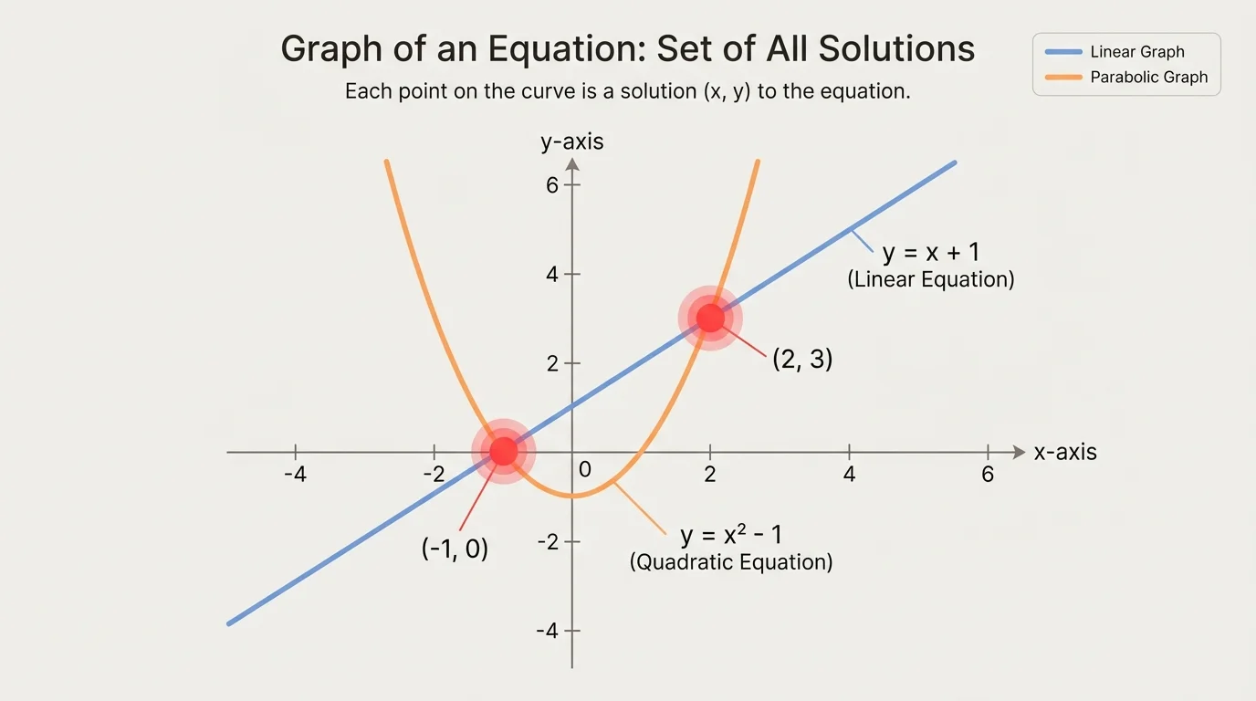
To understand why, suppose the graphs intersect at \(( -1, 0 )\). Substituting into the first equation gives \(0 = -1 + 1\), true. Substituting into the second gives \(0 = (-1)^2\), false, so that point would not actually work. A real intersection must satisfy both equations. Try \((1,1)\): for the first equation, \(1 = 1 + 1\) is false, so that is not a common solution either. The actual common solutions come from points that lie on both graphs simultaneously.
If a line and a parabola cross twice, the system has two solutions. If they touch once, it has one solution. If they never meet, it has no solution. The graph gives a visual answer to the question "Which ordered pairs make both equations true?"
This idea connects directly to earlier work on systems of equations. Instead of solving only by substitution or elimination, you can also solve by graphing and identifying the common solution set. Looking again at [Figure 3], the highlighted intersections represent exactly that shared truth.
Graphs of equations matter outside the classroom because many real situations involve two changing quantities. In a business setting, a cost equation such as \(y = 50x + 200\) can relate the number of items produced, \(x\), to total cost, \(y\). Every point on the graph represents a possible production level and its matching cost.
In physics, the height of a projectile can often be modeled by a quadratic equation, such as \(h = -16t^2 + 64t + 5\). The graph is a curve because height does not change at a constant rate. Each point \((t,h)\) gives a time and a height that fit the motion.
Why graphical representation matters in applications
In real-world modeling, the graph lets you see trends, limits, and key events. A line can show steady growth or decline, while a curve can reveal a maximum, minimum, or turning point. The graph is valuable because it represents all solutions at once rather than one calculation at a time.
Engineers use graphs to compare design constraints. Economists graph supply and demand equations and interpret their intersection. Medical researchers graph data models to study change over time. In each case, the graph is meaningful because it stands for a set of solutions to an equation or a system of equations.
One common mistake is thinking that a graph is only the few points you plotted. Those points are evidence, but the graph represents all solutions, including infinitely many points between the ones you chose, as long as the equation allows them.
Another mistake is reversing coordinates. The point \((2,5)\) is not the same as \((5,2)\). Since substitution depends on using the correct \(x\)-value and \(y\)-value, switching them can change a true solution into a false one.
A third mistake is assuming every equation in two variables gives a line. As we saw earlier with [Figure 2], equations can produce curves such as parabolas or circles. The graph's shape comes from the equation's structure.
"A graph is algebra made visible."
Finally, some students focus only on appearance and forget meaning. A neat sketch is helpful, but what matters most is this: every point on the graph corresponds to a true statement in the equation. That is the core idea that connects graphing, solving, and interpreting equations in two variables.