Two different rules can produce the same output. That simple idea is behind a powerful method in algebra: when two graphs cross, they reveal where two expressions are equal. This matters far beyond a textbook. Engineers compare competing designs, businesses compare cost and revenue, and scientists compare growth and decay models. In each case, the key question is the same: for what value of \(x\) do two quantities match?
Suppose a point lies on both graphs \(y=f(x)\) and \(y=g(x)\). Then both functions give the same \(y\)-value for the same \(x\)-value at that intersection, as [Figure 1] shows. If the point is \((a,b)\), then being on the graph of \(y=f(x)\) means \(f(a)=b\), and being on the graph of \(y=g(x)\) means \(g(a)=b\).
Since both equal \(b\), we must have \(f(a)=g(a)\). That means \(a\), the x-coordinate of the shared point, is a solution of the equation \(f(x)=g(x)\).
Graphical solution means solving an equation by finding where graphs meet on a coordinate plane. For the equation \(f(x)=g(x)\), the solutions are the x-coordinates of the points where the graphs \(y=f(x)\) and \(y=g(x)\) intersect.
The reverse is also true. If \(a\) is a solution of \(f(x)=g(x)\), then the two functions have the same output at \(x=a\). So the point \((a,f(a))\) is also \((a,g(a))\), which means it lies on both graphs. Therefore, solving \(f(x)=g(x)\) and finding intersection points are two views of the same idea.
This is one of the most important links between algebra and graphs. An equation tells you where two expressions are equal. A graph lets you see that equality as a shared point.
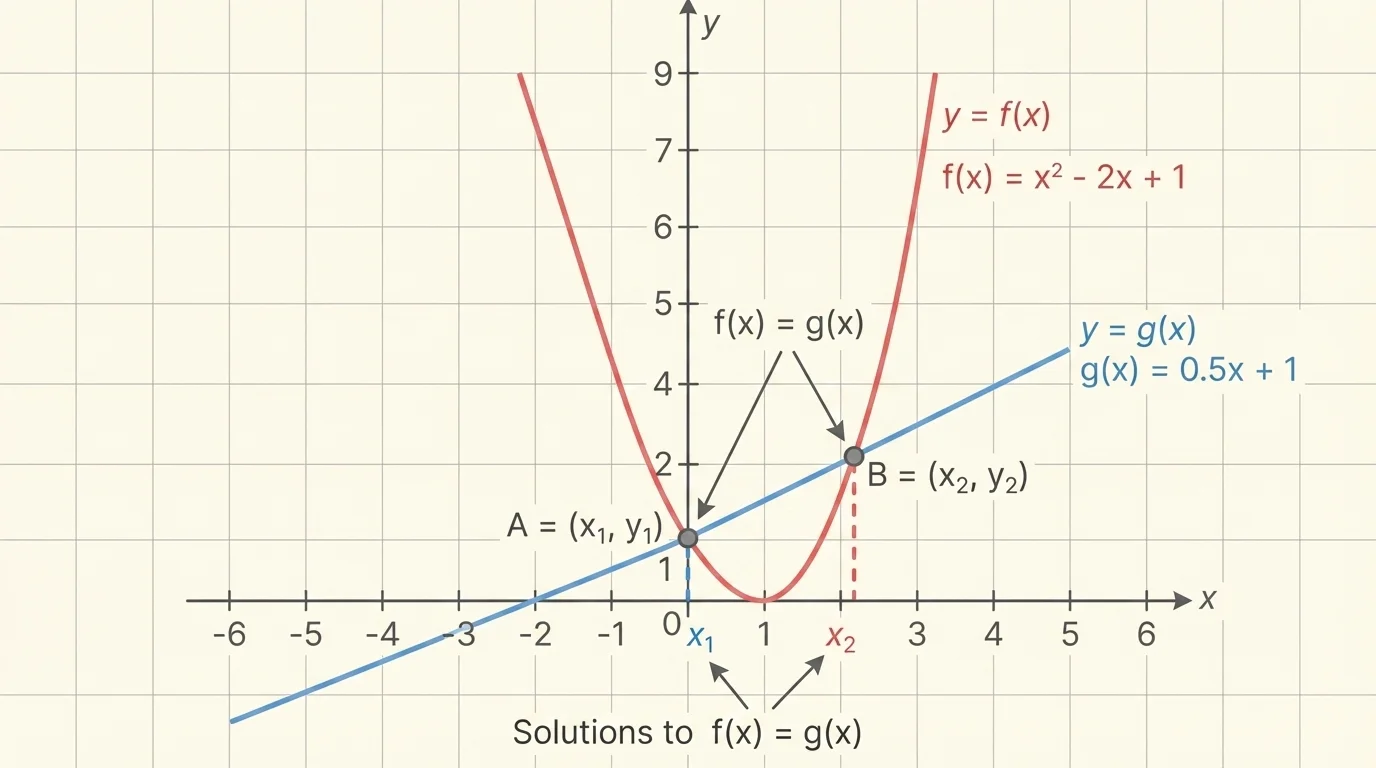
For example, compare \(y=2x+1\) and \(y=x^2-2\). If they intersect, the \(x\)-coordinates of the intersection points satisfy \(2x+1=x^2-2\). Rearranging gives \(x^2-2x-3=0\), so \((x-3)(x+1)=0\). The solutions are \(x=3\) and \(x=-1\). Those are exactly the x-coordinates where the line and parabola meet, just as the shared points in [Figure 1] illustrate.
When you graph two functions, the number of points where they intersect tells you the number of solutions to \(f(x)=g(x)\). If they cross once, there is one solution. If they cross twice, there are two solutions. If they never cross, there is no real solution.
Sometimes a graph gives an exact answer, especially when the intersection lands on a clear grid point such as \((2,5)\). More often, the graph gives an approximate answer, such as \(x\approx 1.7\). Approximation is still valuable. In many real settings, an answer to the nearest tenth or hundredth is enough.
A graph can also show whether a solution is likely to repeat. For example, if a line just touches a parabola without crossing it, there is still an intersection point, but only one distinct \(x\)-value. Algebraically, that often corresponds to a repeated root.
To read a graph accurately, recall that each point has coordinates \((x,y)\). The horizontal coordinate is \(x\), and the vertical coordinate is \(y\). When solving \(f(x)=g(x)\) graphically, the answer is the x-coordinate of each shared point, not the \(y\)-coordinate.
If the graph seems not to intersect, be careful. The viewing window might be too small, the scale might hide a crossing, or one function may not be defined for some values. Good graphing is not just drawing curves; it also means choosing a sensible window and checking the domain.
Many equations cannot be solved easily by hand, or the algebra becomes messy. In those cases, you can still find solutions approximately in three main ways: by graphing with technology, by making tables of values, or by using successive approximations.
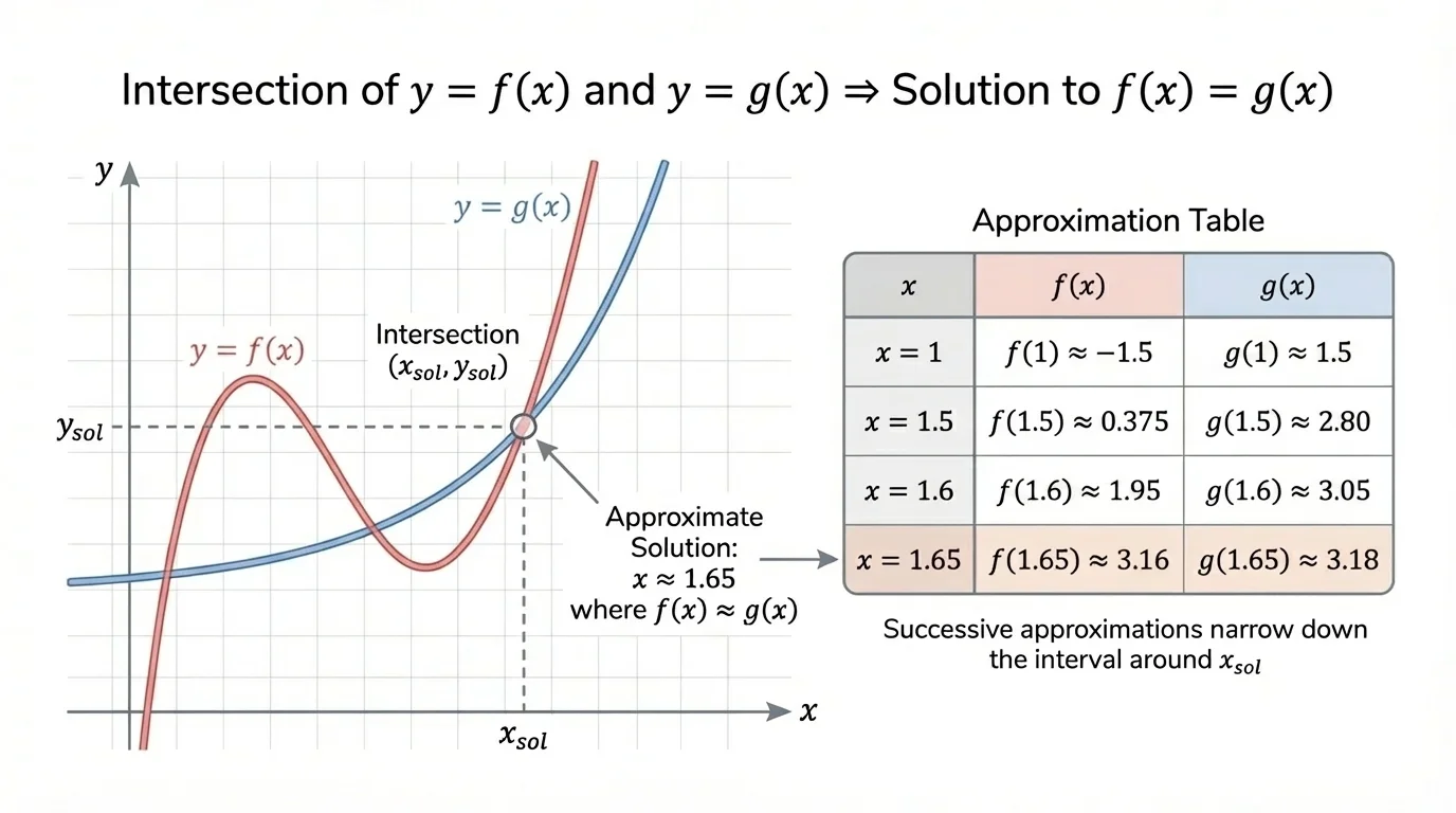
One useful strategy is to define a new function \(h(x)=f(x)-g(x)\). Then solving \(f(x)=g(x)\) is the same as solving \(h(x)=0\). That means you are looking for the zeros of \(h\). If \(h(x)\) changes sign between two nearby \(x\)-values, then a solution lies between them, as [Figure 2] illustrates.
How successive approximation works
Start with an interval where you know a solution lies, such as between \(x=1\) and \(x=2\). Test a value in the middle, like \(x=1.5\). If the two function values are still not equal, decide which half of the interval contains the intersection. Then repeat. Each step narrows the interval and gives a better approximation.
Graphing technology is fast and visual. A graphing calculator or software can plot both functions and estimate the intersection coordinates directly. But technology is most powerful when you understand what it is doing: it is locating where the outputs match.
Tables of values are especially helpful when a graph is not available or when you want to justify an estimate carefully. You choose \(x\)-values, compute \(f(x)\) and \(g(x)\), and look for where one changes from being larger than the other to being smaller.
For instance, if \(f(1)=3\) and \(g(1)=5\), but \(f(2)=7\) and \(g(2)=6\), then at \(x=1\), \(f(x)<g(x)\), while at \(x=2\), \(f(x)>g(x)\). So the graphs must cross somewhere between \(x=1\) and \(x=2\), assuming the functions are continuous there.
Later, when you compare more complicated function families, the narrowing process in [Figure 2] becomes especially useful because exact algebraic solutions may be difficult or impossible to write neatly.
The shape of a graph strongly affects how many solutions \(f(x)=g(x)\) can have. Different function families create different intersection patterns, and [Figure 3] compares some typical cases.
Linear functions have the form \(y=mx+b\). Two different nonparallel lines intersect once, so the equation usually has one solution. Parallel lines do not intersect, so there is no solution. If the lines are the same line, there are infinitely many solutions.
Polynomial functions include quadratics, cubics, and higher powers. A line and a parabola can intersect in \(0\), \(1\), or \(2\) points. Two higher-degree polynomials can have several intersections.
Absolute value functions such as \(y=|x-2|+1\) create a sharp V-shape. A line may cross both arms, touch the vertex, or miss the graph entirely.
Rational functions such as \(y=\dfrac{1}{x-1}\) may have breaks in the graph and asymptotes. They can intersect another graph on one side of an asymptote, both sides, or not at all.
Exponential functions such as \(y=2^x\) grow or decay at changing rates. They often intersect lines or polynomials once or twice, depending on the model.
Logarithmic functions such as \(y=\log(x)\) are only defined for positive inputs in many basic cases, so domain matters immediately. Their intersections with lines or exponentials may need approximation.
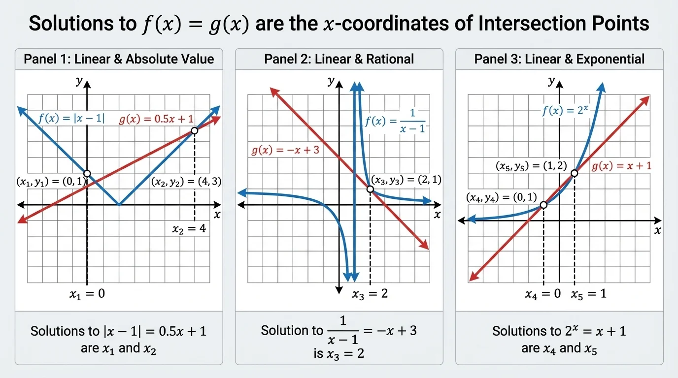
The comparison in [Figure 3] reminds you not to expect every equation to behave like a simple line meeting another line. Sometimes there are several solutions; sometimes none; sometimes the graph's shape or domain rules out values before you even start solving.
The best way to understand graphical solutions is to see them in action across different kinds of functions.
Example 1: Linear and polynomial
Find the solutions of \(x^2=x+2\) by thinking of the graphs \(y=x^2\) and \(y=x+2\).
Step 1: Connect the equation to intersections.
The solutions are the \(x\)-coordinates where the parabola \(y=x^2\) and the line \(y=x+2\) meet.
Step 2: Solve algebraically to confirm the graphical result.
Move all terms to one side: \(x^2-x-2=0\).
Factor: \((x-2)(x+1)=0\).
Step 3: State the solutions.
So \(x=2\) or \(x=-1\).
The graphs intersect at two points, so the equation has two real solutions: \(x=-1,\;2\)
Notice how the graph and the algebra tell the same story. The graph shows two crossings, and the equation produces two solutions.
Example 2: Absolute value and linear
Find the solutions of \(|x-1|=x-3\) approximately or exactly if possible.
Step 1: Interpret as an intersection.
We compare \(y=|x-1|\) and \(y=x-3\).
Step 2: Reason from the graph.
The graph \(y=|x-1|\) is always nonnegative. So we need \(x-3\ge 0\), which means \(x\ge 3\).
Step 3: Solve under that condition.
If \(x\ge 1\), then \(|x-1|=x-1\). So the equation becomes \(x-1=x-3\), which is impossible.
Therefore the graphs do not intersect, so there is no solution. A graph shows the line always below the right arm of the V by \(2\) units.
This example is important because it shows that not every equation has a real solution. A graph can reveal that quickly.
Example 3: Exponential and linear using a table
Find the solution of \(2^x=x+3\) approximately.
Step 1: Compare values.
| \(x\) | \(2^x\) | \(x+3\) |
|---|---|---|
| \(1\) | \(2\) | \(4\) |
| \(2\) | \(4\) | \(5\) |
| \(3\) | \(8\) | \(6\) |
Table 1. Values comparing \(2^x\) and \(x+3\) to locate an intersection.
Step 2: Locate the interval.
At \(x=2\), \(2^x<x+3\). At \(x=3\), \(2^x>x+3\). So a solution lies between \(2\) and \(3\).
Step 3: Narrow the interval.
Try \(x=2.4\): \(2^{2.4}\approx 5.28\), while \(x+3=5.4\). So \(2^{2.4}<x+3\).
Try \(x=2.5\): \(2^{2.5}\approx 5.66\), while \(x+3=5.5\). So \(2^{2.5}>x+3\).
Step 4: Give an approximation.
The solution is between \(2.4\) and \(2.5\), and more careful checking gives about \(x\approx 2.45\).
The graphs intersect once, at approximately \[x\approx 2.45\]
Here, a graphing calculator would estimate the same crossing, but the table method explains why the answer is in that interval.
Example 4: Rational and linear
Find the solutions of \(\dfrac{1}{x}=x\).
Step 1: Think graphically.
The solutions are where \(y=\dfrac{1}{x}\) and \(y=x\) intersect.
Step 2: Solve carefully with the domain in mind.
Multiply both sides by \(x\), but note that \(x\ne 0\): \(1=x^2\).
Step 3: Solve and check.
So \(x=1\) or \(x=-1\). Both are allowed because neither equals \(0\).
The graph has one intersection in quadrant I and one in quadrant III, so \(x=-1,\;1\)
The restriction \(x\ne 0\) matters because \(y=\dfrac{1}{x}\) is undefined there. Rational graphs often demand that extra attention.
Example 5: Logarithmic and linear using successive approximation
Find the solution of \(\log_{10}(x)=1-\dfrac{x}{10}\) approximately.
Step 1: Note the domain.
Because \(\log_{10}(x)\) is defined only for \(x>0\), we look only at positive \(x\)-values.
Step 2: Test values.
At \(x=1\), \(\log_{10}(1)=0\), and \(1-\dfrac{1}{10}=0.9\), so the left side is smaller.
At \(x=5\), \(\log_{10}(5)\approx 0.699\), and \(1-\dfrac{5}{10}=0.5\), so the left side is larger.
Step 3: Narrow the interval.
A solution lies between \(1\) and \(5\). Try \(x=3\): \(\log_{10}(3)\approx 0.477\), and \(1-0.3=0.7\), so the left side is smaller.
Try \(x=4\): \(\log_{10}(4)\approx 0.602\), and \(1-0.4=0.6\), so the values are very close.
Step 4: Refine.
At \(x=3.98\), \(\log_{10}(3.98)\approx 0.600\), and \(1-0.398=0.602\).
At \(x=4.02\), \(\log_{10}(4.02)\approx 0.604\), and \(1-0.402=0.598\).
So the solution is approximately \[x\approx 4.00\]
This last example is exactly the kind of equation where graphing and approximation are more practical than algebraic manipulation.
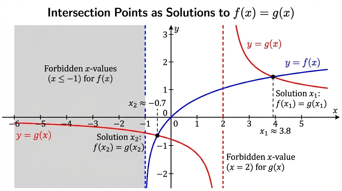
One major idea is domain. A value of \(x\) can only be a solution if both functions are defined there. For example, if one function is \(\dfrac{1}{x-2}\), then \(x=2\) can never be a solution because the function is undefined. The restrictions and asymptotic behavior in [Figure 4] make this visible.
Another key idea is the role of an asymptote. Rational and logarithmic functions may approach a line without touching it. A graph may look close to intersecting near an asymptote, but "very close" is not the same as equal.
Scale also matters. A graph viewed with a poor window can hide intersections or suggest fake ones. If a calculator says there is no crossing, try zooming out or changing the scale before concluding there is no real solution.
Repeated solutions can also occur. If two graphs touch at one point and turn away, the equation still has a solution there, but the graphs do not cross through each other. This often happens when a line is tangent to a parabola.
When checking approximate answers, substitute back into both functions. If the outputs are nearly equal, your estimate is reasonable. This habit helps catch errors caused by graph-reading or rounding.
Later, if you solve the same problem algebraically, the picture from [Figure 4] still helps you judge whether every algebraic result actually makes sense in the domain of the original functions.
Graphs intersect whenever two changing quantities become equal, so this topic has many practical uses.
In business, a company may compare cost and revenue. If cost is modeled by \(C(x)\) and revenue by \(R(x)\), then the break-even point happens when \(C(x)=R(x)\). Graphically, it is where the two graphs intersect. The corresponding \(x\)-value might represent the number of items sold.
In science, one model may describe cooling and another may describe a target temperature. Solving \(T_1(t)=T_2(t)\) tells when the two temperatures match. If one model is exponential, a graph can estimate the time even when an exact formula is awkward.
Air pressure, population growth, medicine concentration in the body, and sound intensity often involve exponential or logarithmic relationships. That is one reason graphical solving is so useful: real models are not always simple polynomials.
In economics, one graph might represent demand and another supply. Their intersection gives the equilibrium quantity. In physics, two motion graphs can be set equal to find when two objects are at the same height or position.
Even in digital technology, signal strength and error rate can be modeled by different functions. Engineers often care most about where the curves meet, because that is the threshold where one behavior gives way to another.
"Algebra is the language of equality; graphs are the picture of it."
Seeing equations and graphs as partners makes mathematics more powerful. The equation gives precision, and the graph gives insight.