A playlist has a first song, a second song, a third song, and so on. A savings account may record its balance after month \(1\), month \(2\), month \(3\), and so on. In both cases, the output depends on a numbered position. That is exactly the idea behind a sequence: instead of plugging any real number into a rule, we usually plug in positive integers or nonnegative integers. This makes sequences one of the clearest ways to see that a function does not need to have all real numbers as inputs.
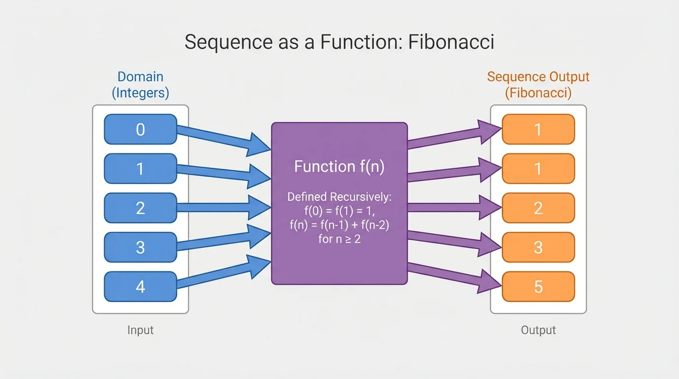
In algebra, students often meet functions written as \(y = f(x)\), where \(x\) can vary continuously. A sequence is different. Its inputs are usually integers such as \(0,1,2,3,\dots\) or \(1,2,3,4,\dots\), and each input gives exactly one output. So a sequence is a special kind of function, and recognizing that fact helps connect patterns, formulas, graphs, and recursive thinking, as [Figure 1] shows.
A sequence is an ordered list of values that follows a rule. The order matters. The first term, second term, third term, and so on are tied to input values, and each input has only one output. That is why a sequence is a function, with integer inputs matched to specific outputs.
If we write a sequence as \(a_1, a_2, a_3, \dots\), then \(a_n\) means the term at position \(n\). We can also use function notation and write \(f(n)\). For example, if \(f(n) = 2n + 1\), then \(f(1) = 3\), \(f(2) = 5\), and \(f(3) = 7\). The same idea could be written as \(a_n = 2n + 1\).
Because each input value corresponds to exactly one term, a sequence satisfies the definition of a function. The main difference is that the inputs are not usually all real numbers. Instead, they come from a counting set such as \(\{1,2,3,4,\dots\}\) or \(\{0,1,2,3,\dots\}\).
Sequence means a function whose domain is a subset of the integers, usually nonnegative integers or positive integers, and whose outputs are listed in order.
Term means one output of the sequence, such as \(a_4\) or \(f(7)\).
Domain means the set of allowed inputs.
Range means the set of resulting outputs.
It is important not to confuse the value of a term with its position. In the sequence \(3,6,9,12,\dots\), the third term is \(9\), not \(3\). The input is the position \(3\), and the output is the value \(9\).
The domain of a sequence is usually a subset of the integers. Many sequences begin with \(n = 1\), so the domain is \(\{1,2,3,\dots\}\). Others begin with \(n = 0\), so the domain is \(\{0,1,2,3,\dots\}\). Which starting point is used depends on how the sequence is defined.
For example, if a sequence counts the number of tiles in a growing pattern starting from a first figure, then \(n = 1\) often makes sense. If a sequence models a situation at the very beginning, such as time \(0\), then starting with \(n = 0\) is natural.
Some sequences can even have domains that include negative integers, although that is less common in introductory algebra. For instance, the rule \(f(n) = n^2\) still makes sense for \(n = -3,-2,-1,0,1,2,3\). But in many school settings, when we say "sequence," we usually mean a function on nonnegative or positive integers.
You already know that a function assigns exactly one output to each input. Sequences follow the same rule. The difference is not the meaning of function; it is the kind of inputs allowed.
This restricted domain is why sequences are often used to model step-by-step change. Months, years, game rounds, terms in a pattern, and stages of a process all naturally use integer inputs rather than every possible real number.
An explicit formula gives the value of a term directly from its position. You do not need earlier terms to calculate the next one. If \(a_n = 4n - 1\), then you can find \(a_{10}\) immediately by substituting \(n = 10\).
Two common families of sequences are arithmetic and geometric sequences. An arithmetic sequence changes by adding the same amount each time. A geometric sequence changes by multiplying by the same factor each time.
| Type of sequence | Example rule | First terms | Pattern |
|---|---|---|---|
| Arithmetic | \(a_n = 3n + 2\) | \(5,8,11,14,\dots\) | Add \(3\) |
| Geometric | \(a_n = 2 \cdot 3^{n-1}\) | \(2,6,18,54,\dots\) | Multiply by \(3\) |
| Quadratic pattern | \(a_n = n^2\) | \(1,4,9,16,\dots\) | Square the index |
Table 1. Examples of explicit formulas for several kinds of sequences.
Explicit rules are useful when you want a term far out in the sequence. For example, finding \(a_{100}\) is easy if you have an explicit formula. You simply evaluate the rule at \(n = 100\).
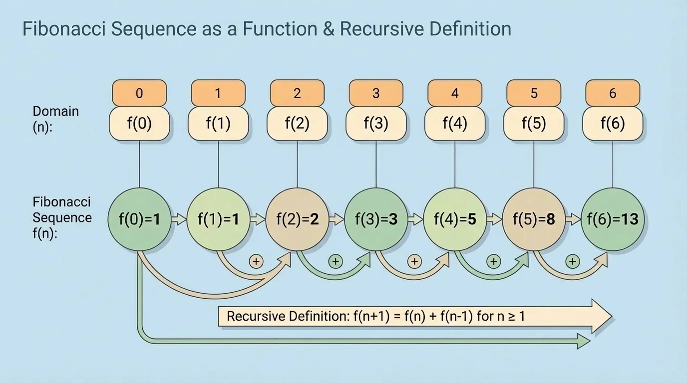
A recursive definition defines each term using one or more earlier terms. Instead of jumping directly to \(a_{50}\), you build the sequence step by step. To make a recursive definition work, you must know at least one starting value, often called an initial condition. This idea is especially clear in the Fibonacci sequence, as [Figure 2] later shows.
For example, consider the sequence defined by \(a_1 = 2\) and \(a_n = a_{n-1} + 3\) for \(n \geq 2\). This means the first term is \(2\), and each new term is \(3\) more than the term before it. So the sequence is \(2,5,8,11,14,\dots\).
Recursive rules are powerful because many real processes depend on what happened one step earlier. Loan balances, populations, repeated investments, and computer algorithms often update from one stage to the next using previous results.
Why recursive rules need starting values
If a rule says "the next term equals the previous term plus \(3\)," that instruction is not enough by itself. You still need to know where the sequence begins. Without an initial term such as \(a_1 = 2\), there would be infinitely many possible sequences that fit the same update rule.
Notice how different recursive and explicit definitions feel. An explicit rule answers "What is the term at position \(n\)?" A recursive rule answers "How do I get from one term to the next?" Both define functions, but they package the information in different ways.
One of the most famous recursively defined sequences is the Fibonacci sequence. It begins with two starting values and then builds each later term from the two before it. Each new term depends on the previous two terms, not just one.
The Fibonacci sequence is defined by the rules
\[f(0) = f(1) = 1, \quad f(n+1) = f(n) + f(n-1)\]
for \(n \geq 1\).
Let us compute the first several terms. We already know \(f(0) = 1\) and \(f(1) = 1\). Then
\(f(2) = f(1) + f(0) = 1 + 1 = 2\), \(f(3) = f(2) + f(1) = 2 + 1 = 3\), \(f(4) = f(3) + f(2) = 3 + 2 = 5\), \(f(5) = f(4) + f(3) = 5 + 3 = 8\), and \(f(6) = f(5) + f(4) = 8 + 5 = 13\).
So the beginning of the sequence is \(1,1,2,3,5,8,13,\dots\). This sequence appears in mathematics, computer science, and models of growth. It is interesting not because every real system follows it exactly, but because it shows how a simple rule can create a rich pattern.
The ratio of consecutive Fibonacci numbers, such as \(\dfrac{13}{8}\), \(\dfrac{21}{13}\), and \(\dfrac{34}{21}\), gets closer and closer to a famous irrational number called the golden ratio.
The Fibonacci example also shows why indexing matters. Here the sequence starts at \(0\), not \(1\). That means the first listed value in the definition is \(f(0)\), and every later calculation must follow that indexing carefully.
Some sequences can be written either explicitly or recursively. For the arithmetic sequence \(2,5,8,11,\dots\), an explicit form is \(a_n = 3n - 1\) for \(n \geq 1\). A recursive form is \(a_1 = 2\) and \(a_n = a_{n-1} + 3\) for \(n \geq 2\).
These two forms describe the same function on the same domain, but they are useful in different situations. The explicit formula is faster for finding a distant term such as \(a_{100}\). The recursive formula highlights the pattern of change from one term to the next.
For Fibonacci numbers, a recursive form is much more natural than a simple explicit one. In fact, there is an explicit formula for Fibonacci numbers, but it is much less intuitive than the recursive definition. That is one reason recursive notation matters so much in higher mathematics.
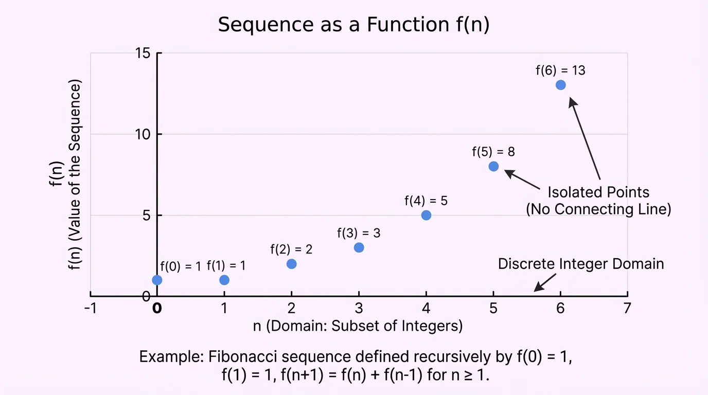
A sequence can be graphed by plotting ordered pairs \((n, a_n)\) or \((n, f(n))\). Because the domain consists of integers, the graph is discrete, not continuous, as [Figure 3] shows. In other words, the graph is a set of separate points rather than a connected curve.
For example, if \(a_n = 2n + 1\) for \(n = 1,2,3,4,5\), then the graph contains the points \((1,3)\), \((2,5)\), \((3,7)\), \((4,9)\), and \((5,11)\). We do not usually connect these points with a line because inputs like \(n = 2.5\) are not part of the domain.
This is a major visual clue that sequences are functions with limited domains. A continuous function such as \(y = 2x + 1\) includes every real \(x\)-value. The corresponding sequence only includes integer inputs. Looking back at Figure 1, the mapping diagram makes the same idea clear in a different representation: only certain input values are allowed.
Graphs of sequences can help you detect growth patterns. If the points rise by equal vertical amounts, the sequence may be arithmetic. If the points rise more and more rapidly, the sequence may be geometric or follow another nonlinear pattern.
The best way to understand sequences as functions is to see how the notation works in actual problems.
Worked example 1
Given the explicit rule \(a_n = 5n - 2\), find \(a_1\), \(a_4\), and \(a_{10}\).
Step 1: Substitute \(n = 1\).
\(a_1 = 5(1) - 2 = 3\).
Step 2: Substitute \(n = 4\).
\(a_4 = 5(4) - 2 = 20 - 2 = 18\).
Step 3: Substitute \(n = 10\).
\(a_{10} = 5(10) - 2 = 50 - 2 = 48\).
The requested terms are
\[a_1 = 3, \quad a_4 = 18, \quad a_{10} = 48\]
This example shows the main advantage of an explicit rule: any term can be found directly from the index.
Worked example 2
A sequence is defined recursively by \(a_1 = 7\) and \(a_n = a_{n-1} - 2\) for \(n \geq 2\). Find the first five terms.
Step 1: Start with the initial condition.
\(a_1 = 7\).
Step 2: Use the recursive rule to get the next terms.
\(a_2 = a_1 - 2 = 7 - 2 = 5\).
\(a_3 = a_2 - 2 = 5 - 2 = 3\).
\(a_4 = a_3 - 2 = 3 - 2 = 1\).
\(a_5 = a_4 - 2 = 1 - 2 = -1\).
The first five terms are
\[7, 5, 3, 1, -1\]
This sequence is arithmetic because the difference between consecutive terms is always \(-2\).
Worked example 3
The Fibonacci sequence is defined by \(f(0) = f(1) = 1\) and \(f(n+1) = f(n) + f(n-1)\) for \(n \geq 1\). Find \(f(2)\), \(f(3)\), \(f(4)\), and \(f(5)\).
Step 1: Use the starting values.
\(f(0) = 1\) and \(f(1) = 1\).
Step 2: Compute each new term from the previous two.
\(f(2) = f(1) + f(0) = 1 + 1 = 2\).
\(f(3) = f(2) + f(1) = 2 + 1 = 3\).
\(f(4) = f(3) + f(2) = 3 + 2 = 5\).
\(f(5) = f(4) + f(3) = 5 + 3 = 8\).
The values are
\[f(2) = 2, \quad f(3) = 3, \quad f(4) = 5, \quad f(5) = 8\]
As seen earlier in [Figure 2], Fibonacci growth is built from repeated addition of the two previous terms.
Worked example 4
Does the rule \(g(n) = \dfrac{1}{n-2}\) define a sequence if the domain is \(\{1,2,3,4,\dots\}\)?
Step 1: Check whether every input in the domain has exactly one output.
At \(n = 1\), \(g(1) = \dfrac{1}{1-2} = -1\), which is well defined.
Step 2: Test the problematic input.
At \(n = 2\), \(g(2) = \dfrac{1}{2-2} = \dfrac{1}{0}\), which is undefined.
Step 3: Decide whether it is a function on the stated domain.
Because one input in the domain does not produce an output, the rule does not define a sequence on that full domain.
If the domain were changed to exclude \(2\), then it could define a sequence on that smaller set.
This last example reminds us that saying "a formula exists" is not enough. The formula must work for every input in the domain.
Sequences appear whenever change happens in steps. A bank account that gains the same amount each month can be modeled by an arithmetic sequence. An account that grows by a fixed percentage each year can be modeled by a geometric sequence. In each case, the input is a whole number of months or years, not every real number in between.
Computer science also uses sequences constantly. Algorithms often repeat instructions step by step, and recursive thinking is essential in programming. The Fibonacci sequence, for example, is a classic case used to teach recursion because each output depends on earlier outputs.
In biology and social science, sequences can model populations measured at regular times. A simple population model might use a recursive rule such as "next year's population equals this year's population plus births minus deaths." Even if real populations are more complicated, sequences give a structured first model.
Engineers and economists also use sequences to analyze repeated growth, decay, and updates. If a quantity is measured at the end of each cycle, then sequence notation naturally fits the situation better than continuous-function notation.
One common mistake is mixing up the index and the term. In \(a_5 = 17\), the input is \(5\) and the output is \(17\). Another common mistake is forgetting where the indexing starts. A sequence beginning with \(f(0)\) works differently from one beginning with \(a_1\).
A second mistake is drawing a connected line through sequence points. Because the graph is discrete, only the integer-input points belong to the sequence. This is why [Figure 3] matters: it emphasizes that a sequence is not usually interpreted as filling in all points between two terms.
A third mistake is trying to use a recursive rule without initial conditions. If you know only that \(a_n = a_{n-1} + 4\), you still do not know the actual sequence until a starting term is given.
Finally, remember that sequences are functions, but they are a special kind of function. Their limited integer domain changes how we write them, graph them, and interpret them. Once you recognize that, explicit rules, recursive rules, and famous examples like Fibonacci all fit into one coherent idea.