Every election season, news reports announce poll results based on a few hundred or a few thousand people, even though millions may vote. That seems almost unbelievable at first: how can a small group say anything useful about a huge population? The answer is one of the central ideas of statistics. Statistics is not just about collecting numbers; it is a process for using data from a carefully chosen part of a population to make informed conclusions about the whole.
In many real situations, measuring every member of a population is impossible, too expensive, or takes too much time. A company that makes light bulbs cannot test every bulb until it burns out before selling it. A medical researcher cannot instantly measure every person in a country. A school principal who wants to know the average number of hours students sleep may not be able to ask every student and verify every answer.
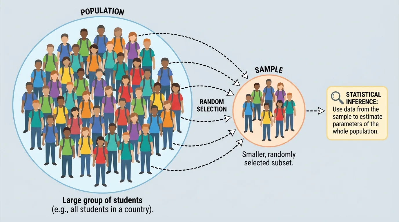
Instead, statisticians collect a sample, which is a smaller group taken from the larger population. If that sample is chosen well, it can provide useful information about the population. The goal is not magic and not perfect certainty. The goal is to make a reasonable inference based on evidence.
This idea appears everywhere: streaming platforms estimate what viewers prefer, doctors study treatment effects, manufacturers monitor product quality, and scientists estimate characteristics of ecosystems. In each case, they use part of a group to learn about the whole group.
Population is the entire group that a study is about.
Sample is the part of the population that is actually observed.
Inference is a conclusion about a population based on sample data.
Good statistical thinking begins with a simple question: Who do we want to know about, and who did we actually measure? If those two groups are mixed up, the conclusion can be misleading.
When statisticians study a population, they often care about a numerical feature of that population, such as an average or a proportion. That true population value is called a parameter. Because measuring the whole population is often unrealistic, we usually do not know the parameter exactly.
Instead, we calculate a value from the sample. A numerical summary of the sample is called a statistic. The statistic is known because it comes from collected data, and it is used to estimate the parameter.
For example, suppose a city wants to know the proportion of all teenagers who wear seat belts every time they ride in a car. The population is all teenagers in the city. The parameter is the true population proportion, which we might call \(p\). If the city surveys a sample of \(200\) teenagers and finds that \(172\) say they always wear a seat belt, then the sample proportion is
\[\hat{p} = \frac{172}{200} = 0.86\]
Here, \(\hat{p} = 0.86\) is a statistic. It gives an estimate of the unknown parameter \(p\).
A useful way to remember the difference is this: a parameter describes the population, while a statistic describes the sample.
| Idea | Describes | Usually Known or Unknown? | Example |
|---|---|---|---|
| Population | Entire group | Known as a group, but not always fully measured | All students in a high school |
| Sample | Part of the group | Known because it is observed | 200 selected students |
| Parameter | Numerical feature of population | Usually unknown | True average sleep time of all students |
| Statistic | Numerical feature of sample | Known after calculation | Average sleep time of the 200 selected students |
Table 1. Comparison of the main ideas used in statistical inference.
A sample can only support a trustworthy conclusion if it is selected in a sensible way. [Figure 1] This is why random sample sampling methods are so important. In a random sample, chance is used to select participants, and each member of the population has a known chance of being chosen. This matters because random selection helps the sample reflect the population when a smaller group is drawn from a much larger one.
If a survey asks only students in the school parking lot at \(7{:}00\) in the morning, it may overrepresent athletes, early arrivals, or students with transportation access. That sample may miss important parts of the student body. A random sample is not perfect, but it reduces the chance of systematic favoritism.
This is the key idea: random sampling gives probability a role in how the sample is chosen. Because of that, statisticians can study how likely it is for sample results to differ from the population. Without a random process, there is no strong mathematical reason to trust the sample as a fair basis for inference.
Why randomness supports inference
When chance selects the sample, no person or group is intentionally favored. That does not guarantee a perfect miniature of the population, but it makes the sample more likely to be representative. It also allows statisticians to analyze the natural variation that comes from sampling.
Random sampling is different from random assignment. Random sampling helps us generalize from a sample to a population. Random assignment is used in experiments to create fair treatment groups. One helps with inference about a population; the other helps with cause-and-effect conclusions in experiments.
[Figure 2] Even when a sample is chosen randomly, the sample statistic will usually not match the population parameter exactly. If you take one random sample and then another, you should expect slightly different results. This idea is called sampling variability. Repeated random samples from the same population produce different statistics.
Suppose the true proportion of students at a school who prefer later start times is \(0.70\). One random sample of \(100\) students might give \(0.66\). Another might give \(0.72\). Another might give \(0.75\). These are not contradictions. They are the expected results of chance.
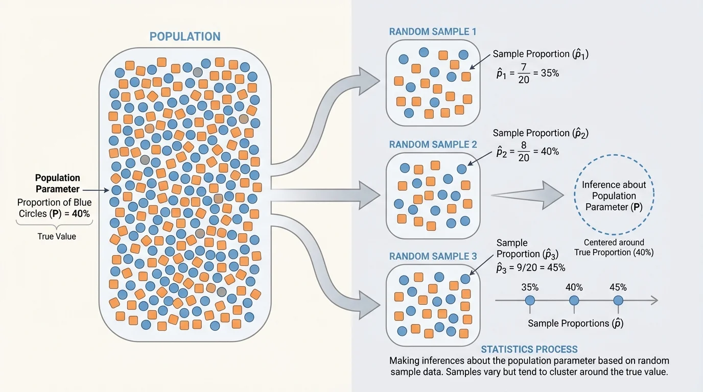
The important pattern is that random samples tend to cluster around the true population value. Some are low, some are high, but a good random process does not push the results consistently in one direction. That is very different from a biased method, which can regularly miss the truth in the same way.
Sampling variability also explains why larger samples are usually more reliable. A sample of \(20\) people may swing widely from one sample to another. A sample of \(2{,}000\) people usually varies much less. Bigger samples do not remove uncertainty, but they often reduce it.
Many national polls can estimate public opinion quite well without surveying millions of people. What matters most is not surveying everyone, but using a large enough random sample and a strong sampling method.
Variation from sample to sample is normal. Statistics is built around understanding that variation rather than pretending it does not exist.
Once a statistic is calculated, statisticians use it as an estimate of the parameter. This is the basic process of statistical inference:
Choose a population. Decide what full group you want to understand.
Select a random sample. Use a method based on chance.
Collect data. Measure the chosen individuals.
Compute a statistic. Find a sample mean, sample proportion, or other summary.
Infer the parameter. Use the statistic to make a conclusion about the population, while recognizing uncertainty.
Suppose a nutrition researcher wants the average number of servings of vegetables eaten per day by teenagers in a district. The true population average is the parameter, often written as \(\mu\). A random sample of \(80\) teenagers gives a sample mean of \(\bar{x} = 2.4\) servings. The researcher might use \(2.4\) as an estimate of \(\mu\), but should remember that another random sample might produce \(2.2\) or \(2.6\).
Inference is therefore a balance of two ideas: using data to estimate the unknown, and respecting the uncertainty caused by chance variation.
The average is found by adding the values and dividing by the number of values. A proportion is the part out of the whole, often written as a decimal or percent. These earlier ideas become powerful in statistics because they are used as sample statistics to estimate population parameters.
The following examples show how a statistic is used to estimate a parameter and how sampling ideas affect the interpretation.
Worked example 1: Estimating a population proportion
A random sample of \(150\) students is asked whether they have a part-time job. In the sample, \(57\) say yes. Estimate the population proportion.
Step 1: Identify the sample statistic.
The sample proportion is \(\hat{p} = \dfrac{57}{150}\).
Step 2: Calculate the value.
\[\hat{p} = \frac{57}{150} = 0.38\]
Step 3: Interpret the result.
The estimate of the population proportion is \(0.38\), or \(38\%\).
Based on this sample, about \(38\%\) of all students in the population may have a part-time job.
This result is an estimate, not a guaranteed exact answer. Another random sample might produce a somewhat different percentage.
Worked example 2: Estimating a population mean
A random sample of \(5\) students reports nightly sleep times of \(6\), \(7\), \(8\), \(7\), and \(9\) hours. Find the sample mean and use it to estimate the population mean.
Step 1: Add the sample values.
\(6 + 7 + 8 + 7 + 9 = 37\)
Step 2: Divide by the sample size.
The sample mean is \(\bar{x} = \dfrac{37}{5} = 7.4\).
Step 3: Interpret the statistic.
Use \(\bar{x} = 7.4\) hours to estimate the population mean \(\mu\).
So the estimated average sleep time for the full population is \(7.4\) hours per night.
Because the sample is small, this estimate may vary quite a bit from the true population mean. A larger random sample would usually provide a more stable estimate.
Worked example 3: Comparing two random samples
A school wants to estimate the proportion of students who support adding more outdoor seating. One random sample of \(100\) students gives \(62\) in favor. A second random sample of \(100\) students gives \(68\) in favor. Are the results inconsistent?
Step 1: Compute both sample proportions.
First sample: \(\hat{p}_1 = \dfrac{62}{100} = 0.62\)
Second sample: \(\hat{p}_2 = \dfrac{68}{100} = 0.68\)
Step 2: Compare the estimates.
The two estimates differ by \(0.68 - 0.62 = 0.06\), which is \(6\%\).
Step 3: Interpret using sampling variability.
The difference does not automatically mean one sample is wrong. Different random samples often give different statistics.
These results are not necessarily inconsistent; they may both be reasonable estimates of the same population proportion.
This is exactly the kind of variation seen in repeated random sampling. The important question is not whether two samples match perfectly, but whether the method was random and the sample sizes were reasonable.
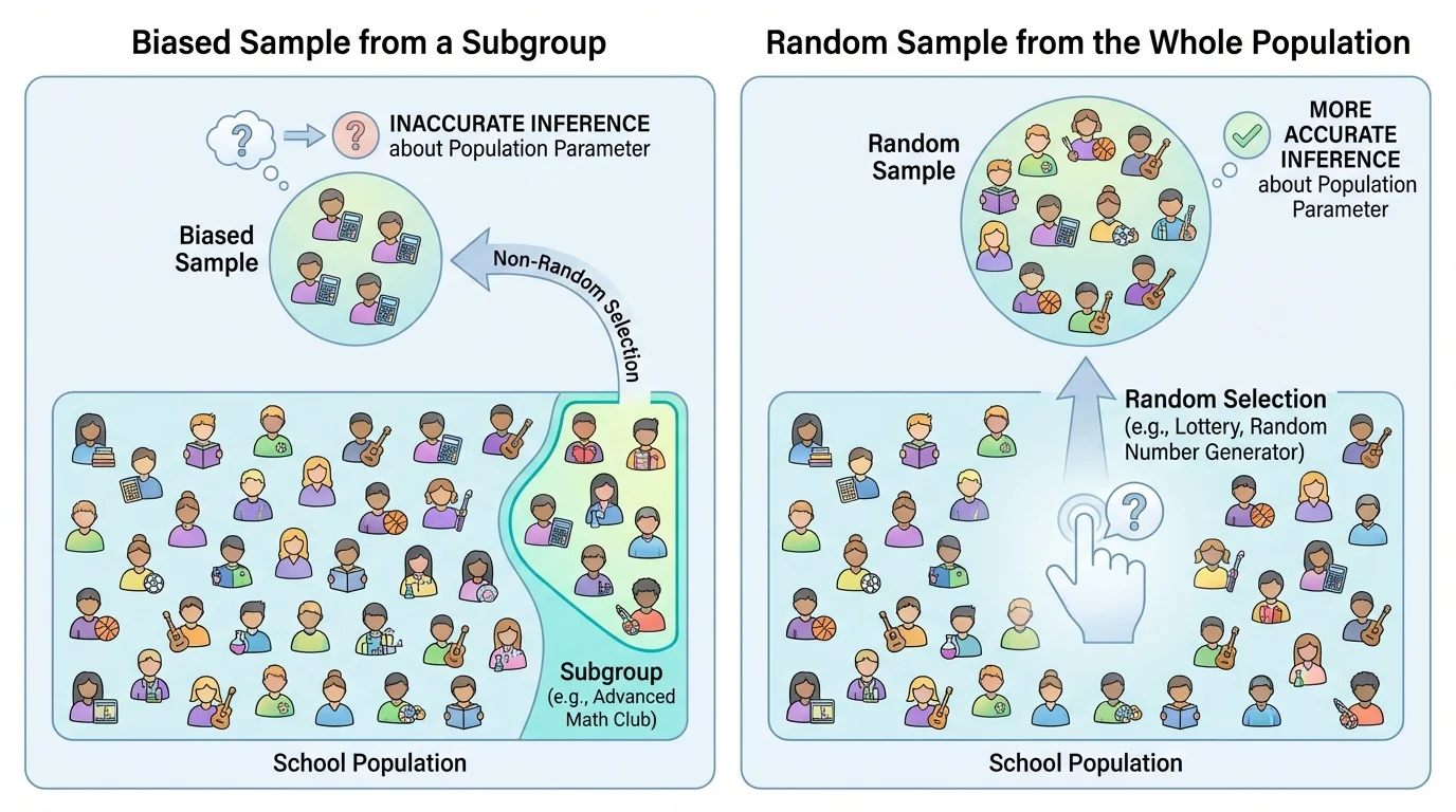
[Figure 3] A statistical conclusion is more believable when the data come from a sound process. A poor sampling method can create bias, which means the method tends to favor certain outcomes. Bias is dangerous because it can systematically push the statistic away from the parameter, especially when one subgroup is oversampled.
For example, if a school surveys only students leaving the gym to estimate how much exercise all students get, the result will probably be too high. That is not just random variation; it is bias caused by the selection method.
Trustworthy inference depends on several ideas:
Random selection: the sample should be chosen by chance.
Representative coverage: the method should give all parts of the population a fair chance to be included.
Adequate sample size: larger random samples usually produce more stable estimates.
Careful measurement: unclear questions or inaccurate data can damage conclusions even if the sample was random.
It is also important to notice what inference can and cannot do. A sample can help estimate a population parameter, but it cannot guarantee exact truth. Statistics deals in evidence and probability, not absolute certainty.
Later, when students study confidence intervals and significance tests, they build on this same idea: random sampling creates a mathematical basis for judging how close a sample statistic may be to the population parameter.
This contrast remains important in advanced work too. A larger biased sample is often worse than a smaller well-randomized sample, because bias does not disappear just by collecting more data.
Public opinion polling: Pollsters use random samples of voters to estimate the proportion who support a candidate or policy. Sampling variability explains why poll results have margins of error and why different polls may differ slightly.
Medicine: Researchers study a sample of patients to estimate how a treatment works in a larger population. If the sample is not representative, the treatment may appear more or less effective than it really is.
Manufacturing: Factories inspect random samples from a production line to estimate defect rates. Testing every item may be too slow or too costly, so sampling supports efficient quality control.
Education: Districts may test a sample of students to estimate average achievement or attendance trends. The usefulness of these conclusions depends heavily on whether the sample was selected fairly.
Sports analytics: A coach may study a sample of plays to estimate shooting percentages, pass completion rates, or average sprint times. Small samples can be misleading, which is why analysts often want larger datasets before making strong claims.
"The sample is the voice we hear; the population is the group we are trying to understand."
That idea captures the heart of inference. We almost never hear from everyone, so the challenge is to make sure the voice we do hear comes from a fair and informative sample.
Statistics is often described as the science of learning from data, but that phrase matters most when we remember where the data came from. A number by itself does not guarantee truth. A sample mean or sample proportion becomes meaningful only when it is connected to a well-defined population and obtained through a random process.
So when you see a headline such as "\(64\%\) of students prefer digital notes" or "average commute time is \(18.5\) minutes," the critical statistical question is not just What is the number? It is also How was the sample chosen, and what population is the claim about?
That habit of questioning the process is what turns statistics from simple calculation into real reasoning.