Suppose a company claims its new energy drink improves reaction time, a teacher says one review method raises test scores, or a farm reports that a new fertilizer increases crop growth. In all of these cases, the big question is the same: is the treatment actually better, or did the difference happen just by chance? Statistics gives us a way to answer that question without guessing.
When researchers run a fair experiment, they often compare treatments, which are the conditions being tested. Then they look at the outcomes and measure the difference between the groups. But seeing a difference is not enough. Even if two treatments are really equally effective, random assignment can still create some difference in the data. That is why we use simulations to decide whether the observed result is large enough to count as meaningful evidence.
This idea is central to statistical reasoning: data from an experiment help us judge whether a difference in a sample reflects a real difference in a population parameter, or whether it is just random variation.
[Figure 1] In a randomized experiment, subjects are randomly assigned to one of two treatments. That random assignment is powerful because it helps balance out other factors that might affect the response. If one group ends up slightly stronger, faster, or more experienced, random assignment makes that due to chance rather than researcher choice.
The outcome being measured is called the response variable. For example, the response variable might be reaction time, test score, plant height, or whether a patient improved. Because the groups were formed randomly, a large difference in outcomes can be used as evidence that the treatment caused the difference.
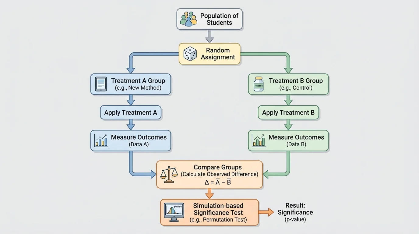
This is different from an observational study, where people choose their own conditions or are simply observed as they are. In an observational study, differences between groups may be caused by hidden factors. In a randomized experiment, random assignment makes a cause-and-effect conclusion much more reasonable.
Randomization does not guarantee perfectly equal groups. One group might still have slightly more experienced students or slightly taller plants. The key point is that these imbalances arise by chance, not bias. Because of that, probability can help us measure how surprising the observed difference really is.
Treatment is a specific condition applied in an experiment. Random assignment means assigning subjects to treatments by chance. Response variable is the outcome measured to see the effect of the treatment. Statistic is a number calculated from sample data, such as a sample mean or sample proportion.
When two treatments are compared, the statistic we often care about is the difference between groups. If the response is categorical, such as success or failure, we compare sample proportions. If the response is numerical, such as test score or growth in centimeters, we compare sample means.
Suppose Treatment A gives a success rate of \(0.62\) and Treatment B gives a success rate of \(0.48\). The observed difference in sample proportions is \(0.62 - 0.48 = 0.14\). That tells us the sample favored Treatment A by \(14\) percentage points.
Or suppose students using one study method score an average of \(84.3\) while students using another method score \(80.1\). Then the observed difference in sample means is \(84.3 - 80.1 = 4.2\) points.
These numbers describe the sample, but they do not automatically prove the treatment effect is real. Why not? Because random assignment itself creates variation. Even if there were no true difference between treatments in the population, one group could still come out ahead in the sample.
So the real question is not "Is the difference exactly zero?" It is "Is the observed difference too large to be explained by chance alone?" That question leads directly to simulation.
Earlier probability work matters here. If chance can create variation in repeated random samples, then chance can also create variation in repeated random assignments. Statistical inference studies whether the observed result is unusual under a chance-only model.
A useful starting point is the null hypothesis. In this setting, it says there is no treatment effect, so the two treatments are equally effective in the population. If that were true, then any difference we see in the experiment would come from random assignment alone.
[Figure 2] To test whether chance alone is a believable explanation, we build a model of what chance would produce. A null model assumes the null hypothesis is true and then uses random reassignment or shuffling to imitate the experiment many times.
Here is the basic idea. Keep the observed outcomes the same, but shuffle the treatment labels. If the null hypothesis is true, the labels "Treatment A" and "Treatment B" should not matter. After shuffling, calculate the difference in proportions or means again. Repeat this many times.
The collection of simulated differences shows what kinds of results are expected from chance alone. Most simulated differences will be near \(0\), but some will be farther away. If the actual observed difference is much more extreme than almost all of the simulated ones, that is evidence against the null hypothesis.
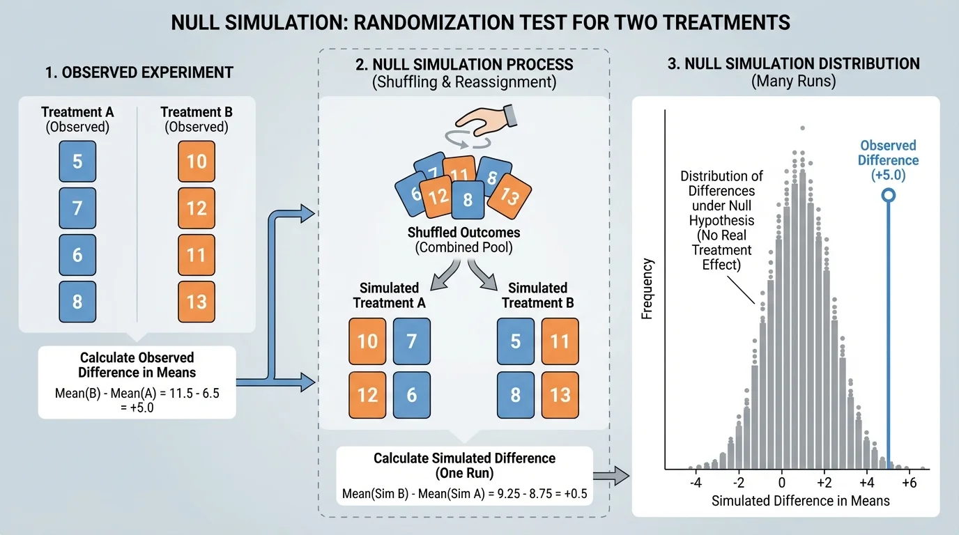
This process is often called a randomization test. Technology makes it practical because a computer can perform hundreds or thousands of shuffles quickly. Even without advanced formulas, simulation lets us reason from probability in a direct and visual way.
The word parameter refers to the true population value, such as the true proportion of success under each treatment or the true mean score under each treatment. We usually do not know the parameters. Instead, we use sample statistics and simulation to judge whether the parameters are likely to differ.
Chance variation and significance
Not every observed difference is meaningful. Random assignment naturally creates some spread in outcomes. A difference is called statistically meaningful when it would be unlikely to occur often in a chance-only world. Simulation helps estimate how rare that result would be.
If the observed result is common in the simulation, then chance alone is a reasonable explanation. If it is rare in the simulation, then the data provide evidence that the treatments differ.
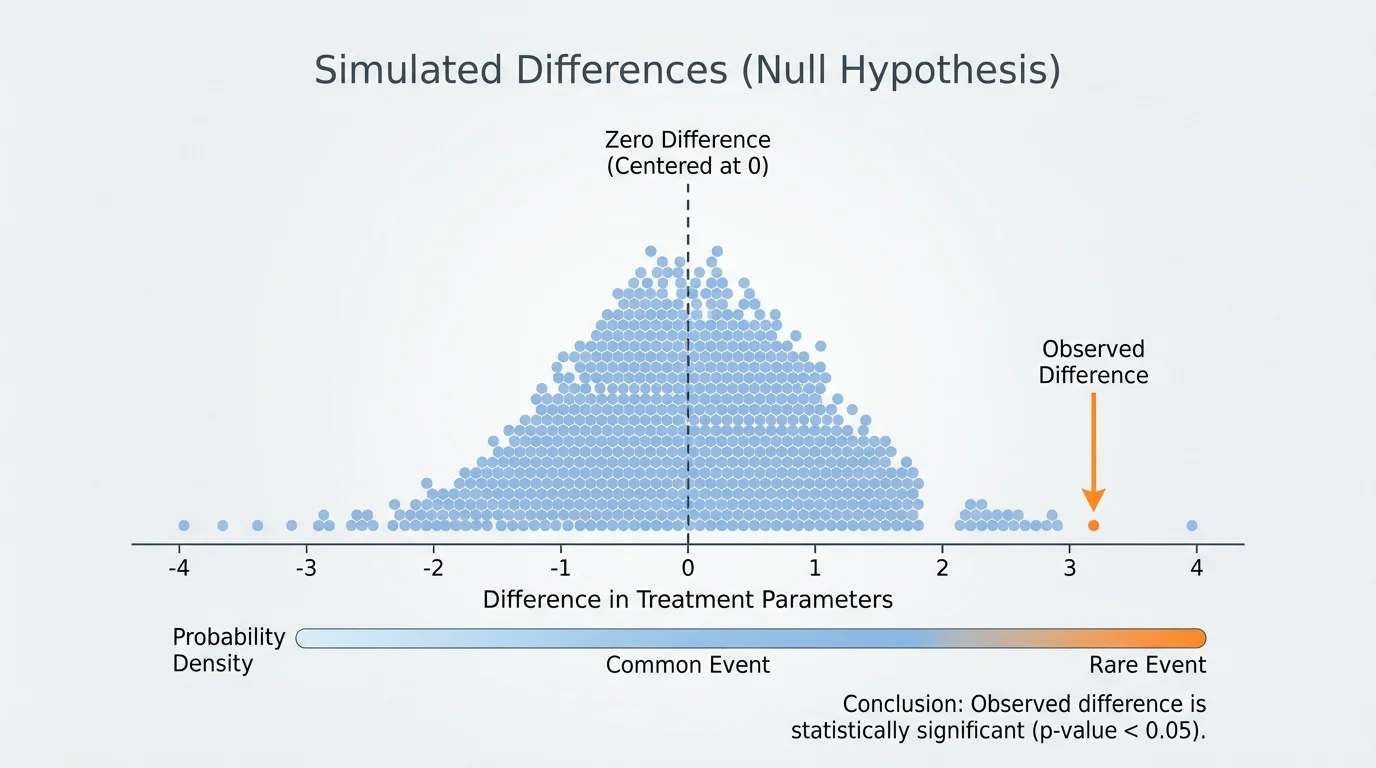
[Figure 3] After many shuffles, we can display the simulated differences in a graph. The distribution is usually centered near \(0\) because the null hypothesis says there is no real treatment effect.
Now place the observed difference on that distribution. If the observed value sits near the center, it is not unusual. If it lies far out in a tail, it is unusual under the null model.
This leads to the idea of a p-value. Informally, the p-value is the proportion of simulated results that are at least as extreme as the observed difference, assuming the null hypothesis is true. A small p-value means the observed result is hard to explain by chance alone.
For example, if only \(2\) out of \(1{,}000\) simulations are as extreme as the observed difference, then the estimated p-value is \(\dfrac{2}{1000} = 0.002\). That is very small, so the result is statistically significant.
If \(210\) out of \(1{,}000\) simulations are at least as extreme, then the estimated p-value is \(\dfrac{210}{1000} = 0.21\). That is not small, so the observed difference is consistent with chance variation.
There is no magical line built into nature, but many studies use \(0.05\) as a benchmark. If the p-value is less than \(0.05\), the result is often called statistically significant. That means the difference is unlikely under the null model, not that the treatment is guaranteed to be important in practice.
A school sports science club randomly assigns \(50\) students to drink an energy drink and \(50\) students to drink water before a reaction-time task. In the energy-drink group, \(34\) students improve. In the water group, \(25\) students improve.
Comparing two proportions
Step 1: Compute the sample proportions.
Energy drink: \(\hat{p}_1 = \dfrac{34}{50} = 0.68\)
Water: \(\hat{p}_2 = \dfrac{25}{50} = 0.50\)
Step 2: Find the observed difference.
\[\hat{p}_1 - \hat{p}_2 = 0.68 - 0.50 = 0.18\]
Step 3: State the null idea.
Assume the drink has no real effect, so both treatments are equally likely to lead to improvement. Then the difference \(0.18\) might have happened by random assignment.
Step 4: Use simulation.
Combine the \(59\) improved and \(41\) not improved outcomes, then randomly reassign \(50\) outcomes to each treatment many times. Each time, calculate the difference in proportions.
Step 5: Interpret the simulation.
Suppose only \(14\) out of \(1{,}000\) simulated differences are at least \(0.18\) in magnitude. Then the estimated p-value is \(0.014\).
Because \(0.014 < 0.05\), the result is statistically significant. The data provide evidence that the population success proportions differ under the energy drink and water treatments.
This does not prove every individual will improve, and it does not tell us whether the drink is healthy or worth using. It only tells us that the experiment gives evidence of a real difference in the population proportions. The reasoning follows the same pattern shown earlier in [Figure 3]: the observed statistic falls in a tail of the chance-only distribution.
A teacher randomly assigns \(24\) students to Method A and \(24\) students to Method B for a vocabulary unit. After the unit test, Method A has a mean score of \(86.5\), and Method B has a mean score of \(81.8\).
Comparing two means
Step 1: Identify the statistic.
Because test score is numerical, compare sample means.
Step 2: Compute the observed difference.
\[\bar{x}_A - \bar{x}_B = 86.5 - 81.8 = 4.7\]
Step 3: Set up the null model.
Assume the study methods are equally effective. Then the \(48\) scores could have been attached to either group label by chance.
Step 4: Simulate repeated random assignments.
Shuffle the \(48\) scores, deal \(24\) to Group A and \(24\) to Group B, and compute the difference in means each time.
Step 5: Make a decision.
Suppose \(31\) out of \(1{,}000\) simulations produce a difference of at least \(4.7\) points in magnitude. Then the estimated p-value is \(0.031\).
Since \(0.031 < 0.05\), the result is statistically significant. There is evidence that the two study methods lead to different mean scores.
Notice that we did not need to assume the difference had to be positive. If the question is whether the methods are different, then "at least as extreme" usually means far from \(0\) in either direction. That is why the tails of the simulation distribution matter.
Random assignment supports a cause-and-effect conclusion here. Because the teacher assigned students randomly, it is reasonable to say the difference in average scores is linked to the study method rather than to preexisting differences between groups.
A greenhouse randomly assigns \(20\) plants to Fertilizer A and \(20\) plants to Fertilizer B. After six weeks, the mean growth is \(18.2\) cm for A and \(17.5\) cm for B.
A small difference that is not significant
Step 1: Compute the observed difference.
\[18.2 - 17.5 = 0.7\]
Step 2: Build the null model.
Assume the fertilizers do not differ in true mean growth. Shuffle the \(40\) growth measurements many times between the two labels.
Step 3: Compare the observed difference to the simulated ones.
Suppose \(287\) out of \(1{,}000\) simulations have a difference of at least \(0.7\) cm in magnitude. Then the estimated p-value is \(0.287\).
Because \(0.287\) is large, the observed difference is not statistically significant. The data do not provide strong evidence that the fertilizers differ in mean growth.
This example matters because many students think "any difference means one treatment is better." That is false. The difference must be judged against what chance alone can create. As the shuffling process in [Figure 2] suggests, some sample differences happen routinely even when there is no true treatment effect.
One major mistake is confusing statistical significance with practical importance. A treatment might produce a statistically significant increase of only \(0.3\) points on a \(100\)-point test. With a large enough sample, even tiny effects can look statistically significant. But that does not mean the effect is useful in real life.
Another mistake is ignoring sample size. Larger samples usually give more stable results and make it easier to detect real differences. Smaller samples create more variability, so even a noticeable observed difference may not be significant.
Bias is also important. Random assignment helps with fair treatment comparison, but poor measurement, nonresponse, or inconsistent procedures can still weaken a study. If one group receives clearer instructions or better equipment, the experiment is no longer comparing only the treatments.
It is also important to state conclusions carefully. If the result is significant, say the data provide evidence of a difference between the population parameters, such as a difference in true means or true proportions. If the result is not significant, do not say the treatments are definitely equal. Instead, say the data do not provide convincing evidence of a difference.
| Situation | What to Compare | Possible Conclusion |
|---|---|---|
| Categorical outcome | Difference in sample proportions, \(\hat{p}_1 - \hat{p}_2\) | Evidence about a difference in population proportions |
| Numerical outcome | Difference in sample means, \(\bar{x}_1 - \bar{x}_2\) | Evidence about a difference in population means |
| Small p-value | Observed statistic is unusual under null model | Statistically significant result |
| Large p-value | Observed statistic is common under null model | Difference may be due to chance |
Table 1. Comparison of common treatment-comparison situations and how conclusions are stated.
Modern clinical trials, online A/B tests, and agricultural field trials all use the same core logic: random assignment creates fair groups, and probability helps decide whether a result is larger than chance would usually produce.
Even though the settings differ, the reasoning is remarkably similar. Whether you are comparing vaccines, teaching strategies, webpage designs, or running shoes, the goal is to separate true treatment effects from random noise in data.
In medicine, researchers randomly assign patients to a new treatment or a standard treatment, then compare recovery rates or average symptom scores. If simulation shows that the observed difference would be rare under equal effectiveness, the new treatment gains evidence in its favor.
In education, schools may compare tutoring programs, reading strategies, or study schedules. In agriculture, scientists compare seeds, fertilizers, or irrigation methods. In sports science, trainers compare warm-up routines or recovery plans. In technology, companies compare two app designs to see which leads to more clicks or longer use.
These applications all depend on the same idea: use data from a randomized experiment to compare two treatments, then use simulation to decide whether the difference between the population parameters is significant. That is how statistics turns raw results into justified conclusions.