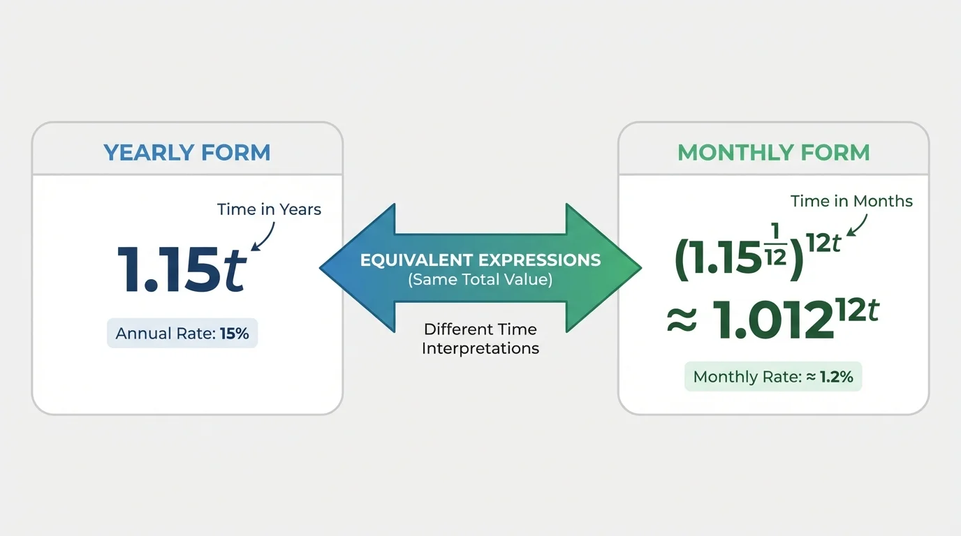
A bank ad might promise 15% annual growth, but your account balance does not wait until New Year's Day to change. Growth often happens in smaller time steps: monthly, daily, even continuously. That is why a single exponential expression can hide useful information until you rewrite it. An exponential function such as \(1.15^t\) tells you the yearly growth factor, but the equivalent form \((1.15^{1/12})^{12t}\) reveals the monthly growth factor. The mathematics has not changed, but the meaning becomes easier to see.
In algebra, rewriting an expression without changing its value is powerful because the new form can highlight a feature that was less obvious before. With exponential expressions, equivalent forms often reveal the rate of growth or decay per different unit of time. This is especially important in finance, population models, medicine, and technology, where rates are often reported in one unit but applied in another.
An equivalent form is a new version of an expression that has the same value as the original expression. For exponential models, changing the form can help answer questions such as: Is the rate monthly or yearly? Is the quantity growing or shrinking? What percent change happens in each smaller time interval?
Suppose an amount grows by \(15\%\) each year. A natural model is
\[A(t) = A_0(1.15)^t\]
where \(A_0\) is the starting amount and \(t\) is measured in years. This form clearly shows annual growth. But if you want to know the monthly growth factor, you can rewrite the same expression using twelfths of a year. The algebra exposes a hidden feature of the quantity.
Growth factor is the number multiplying the amount in each equal time interval. For a growth rate of \(r\), the growth factor is \(1+r\).
Decay factor is the number multiplying the amount in each equal time interval when the quantity decreases. For a decay rate of \(r\), the decay factor is \(1-r\).
Fractional exponent means an exponent such as \(\dfrac{1}{12}\) or \(\dfrac{3}{2}\). It often represents a root or repeated smaller-step growth.
If two expressions are equivalent, they produce the same output for every allowed input. That means the graph, the values, and the modeled situation stay the same. Only the point of view changes.
To rewrite exponential expressions, you need a few key properties of exponents. These are not new formulas to memorize separately from meaning; they are the tools that let you reveal structure.
The most important exponent properties here are
\[a^{mn} = (a^m)^n = (a^n)^m\]
and
\[a^{m+n} = a^m \cdot a^n\]
for positive bases \(a\). When working with time units, the first property matters most because it lets you split one exponent into two parts.
For example, if \(t\) is in years, then \(t = \dfrac{12t}{12}\). So
\[1.15^t = 1.15^{\frac{12t}{12}} = \left(1.15^{1/12}\right)^{12t}\]
This says that growing by a factor of \(1.15\) over one year is equivalent to growing by a factor of \(1.15^{1/12}\) over each month, repeated \(12t\) times.
Recall that a percentage increase of \(15\%\) does not mean the base is \(15\). It means the base is \(1 + 0.15 = 1.15\). Likewise, a decrease of \(8\%\) means the base is \(1 - 0.08 = 0.92\).
Fractional exponents are especially useful here. The expression \(a^{1/12}\) is the twelfth root of \(a\). In growth models, it represents the factor for one month when \(a\) is the factor for one year.
Equivalent forms can highlight different time scales, as [Figure 1] illustrates with yearly and monthly interpretations of the same exponential model. The key idea is to write the exponent in a way that matches the unit you want. If a function is written with years but you want months, replace \(t\) with \(\dfrac{12t}{12}\) and then use the power-of-a-power property.
Start with a general exponential expression:
\(b^t\)
If you want to express the same growth in \(n\) smaller intervals per unit time, rewrite it as
\[b^t = \left(b^{1/n}\right)^{nt}\]
This is one of the most useful transformations in exponential modeling. It does not change the function. It only changes what the base tells you.
For example, yearly growth can be rewritten as monthly growth, quarterly growth, or daily growth. If a quantity triples every year, then \(3^t\) can be rewritten as \((3^{1/12})^{12t}\) to show monthly growth or \((3^{1/4})^{4t}\) to show quarterly growth.
The same idea works in reverse. If you know a monthly factor \(m\), then a yearly factor is \(m^{12}\). So monthly and yearly forms are connected by roots and powers.
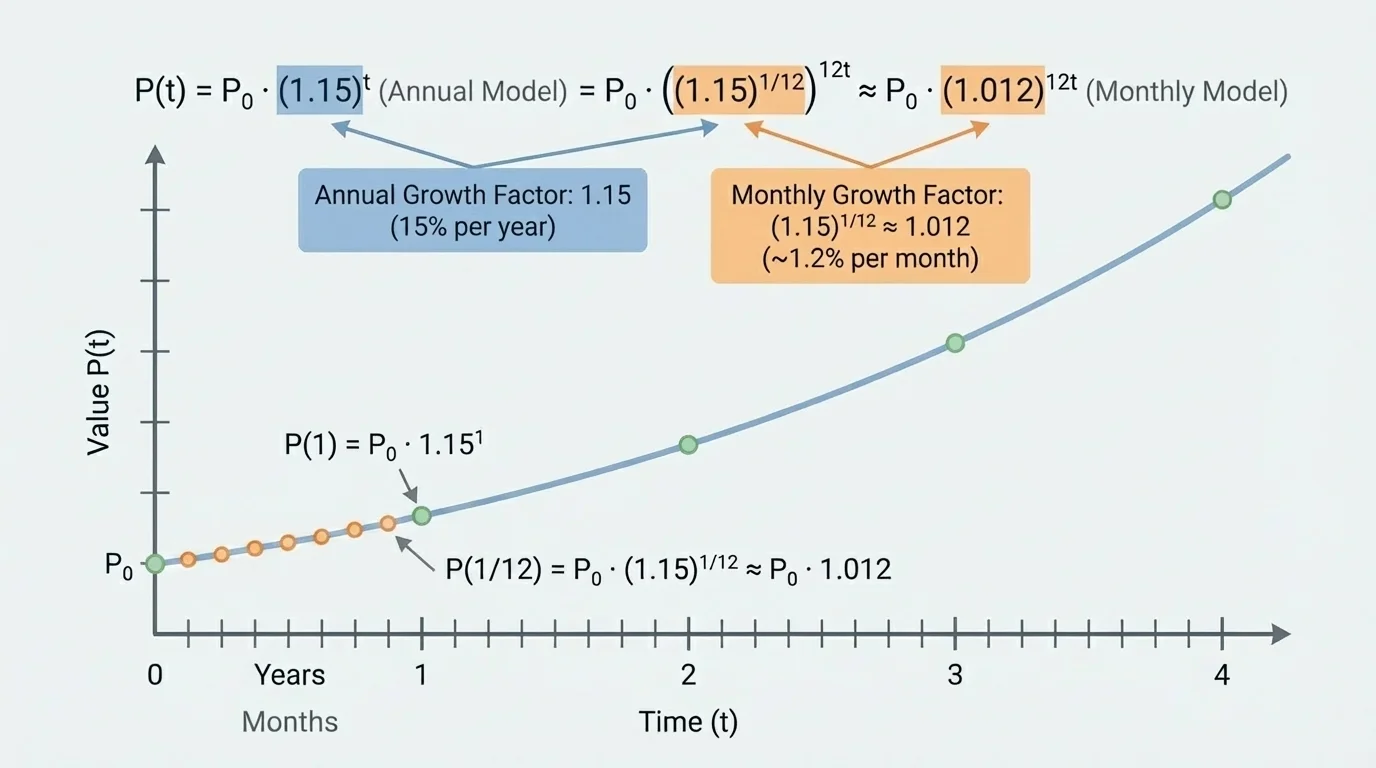
When the yearly growth factor is known, the monthly factor is the twelfth root of that yearly factor. [Figure 2] shows how the graph of the same function can be interpreted with different time units through annual checkpoints and monthly subdivisions on one growth curve. This is exactly what happens in the expression
\[1.15^t = \left(1.15^{1/12}\right)^{12t}\]
Now approximate the monthly factor:
\[1.15^{1/12} \approx 1.0117\]
This means the amount grows by a factor of about \(1.0117\) each month. To convert that factor to a monthly percent increase, subtract \(1\):
\[1.0117 - 1 = 0.0117\]
So the approximate monthly interest rate is about \(1.17\%\), not \(\dfrac{15\%}{12} = 1.25\%\). That difference matters because exponential growth compounds. Equal division of the annual percentage does not produce the same total growth over the year.
This is an important idea in finance: a nominal annual rate and an effective monthly rate are not found by simple division unless the model is linear. Exponential models grow by multiplication, so roots and powers are the correct tools.
A credit card, savings account, or student loan may report rates in one time unit while calculations happen in another. Understanding equivalent exponential forms helps you read the real meaning behind the numbers.
We can generalize this process. If the annual factor is \(a\), then the monthly factor is \(a^{1/12}\). If the annual factor is \(0.90\), meaning a \(10\%\) yearly decrease, then the monthly decay factor is \(0.90^{1/12}\).
Worked example 1
Rewrite \(1.15^t\) to reveal the monthly growth factor, and estimate the monthly percent increase.
Step 1: Split one year into \(12\) months.
Write \(t\) as \(\dfrac{12t}{12}\): \(1.15^t = 1.15^{\dfrac{12t}{12}}\).
Step 2: Use the power-of-a-power property.
\(1.15^{\dfrac{12t}{12}} = \left(1.15^{1/12}\right)^{12t}\).
Step 3: Approximate the new base.
\(1.15^{1/12} \approx 1.0117\).
Step 4: Interpret the factor as a rate.
Monthly rate \(\approx 1.0117 - 1 = 0.0117 = 1.17\%\).
The equivalent form is \(\left(1.15^{1/12}\right)^{12t} \approx (1.0117)^{12t}\), which reveals an approximate monthly increase of \(1.17\%\).
This example shows why equivalent forms are useful: the original form tells you yearly growth, while the new form tells you monthly growth without changing the actual model.
Worked example 2
A population doubles every \(3\) years. The model is \(P(t) = P_0 \cdot 2^{t/3}\), where \(t\) is in years. Rewrite the expression to reveal the yearly growth factor.
Step 1: Notice that \(2^{t/3} = \left(2^{1/3}\right)^t\).
This follows from \(a^{mn} = (a^m)^n\).
Step 2: Approximate the base.
\(2^{1/3} \approx 1.2599\).
Step 3: Interpret the result.
The yearly growth factor is about \(1.2599\), so the yearly growth rate is about \(25.99\%\).
The equivalent form is \(P(t) = P_0(1.2599)^t\), which reveals the approximate yearly growth rate.
Notice how the rewritten form answers a new question. The original model emphasizes doubling every three years; the new form emphasizes the approximate annual increase.
Worked example 3
Rewrite \(500(0.82)^t\) to show the quarterly decay factor, assuming \(t\) is measured in years.
Step 1: Split each year into \(4\) quarters.
\((0.82)^t = \left(0.82^{1/4}\right)^{4t}\).
Step 2: Approximate the quarterly factor.
\(0.82^{1/4} \approx 0.9516\).
Step 3: Interpret the factor.
Since \(0.9516 < 1\), this is decay. The quarterly decrease is about \(1 - 0.9516 = 0.0484 = 4.84\%\).
The equivalent form is \(500(0.9516)^{4t}\), which reveals an approximate quarterly decrease of \(4.84\%\).
This example shows that the same exponent rules work for decay as well as growth. The only difference is that the base is between \(0\) and \(1\).
Worked example 4
A bacterial culture grows according to \(N(t) = 800(1.06)^{2t}\), where \(t\) is in hours. Rewrite it to show the growth factor per hour.
Step 1: Use the rule \(a^{mn} = (a^m)^n\).
\((1.06)^{2t} = \left((1.06)^2\right)^t\).
Step 2: Square the base.
\((1.06)^2 = 1.1236\).
Step 3: Rewrite the model.
\(N(t) = 800(1.1236)^t\).
Step 4: Interpret the meaning.
The factor per hour is \(1.1236\), so the hourly growth rate is \(12.36\%\).
The new form reveals the factor per hour because the original expression applied the growth factor \(1.06\) twice each hour.
As these examples show, transforming exponential expressions is not just symbol manipulation. It changes what the expression tells you about the situation.
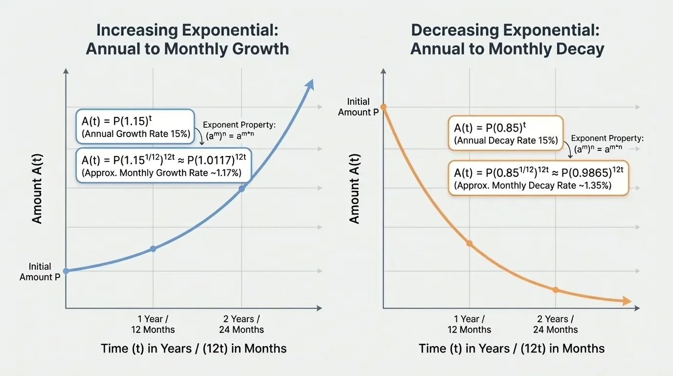
Whether an exponential model represents increase or decrease depends on the base, and [Figure 3] makes this visible by comparing equivalent forms of growth and decay side by side. If the base is greater than \(1\), the function shows growth. If the base is between \(0\) and \(1\), it shows decay.
These ideas can be organized clearly:
| Type of model | General form | Meaning of base |
|---|---|---|
| Growth | \(A_0(1+r)^t\) | Base is greater than \(1\); quantity increases by rate \(r\) each interval |
| Decay | \(A_0(1-r)^t\) | Base is between \(0\) and \(1\); quantity decreases by rate \(r\) each interval |
| Equivalent smaller-step form | \(A_0\left((1+r)^{1/n}\right)^{nt}\) | Base shows the factor for each smaller interval |
Table 1. Comparison of exponential growth, decay, and equivalent forms using different time intervals.
If you rewrite \((1+r)^t\) as \(((1+r)^{1/n})^{nt}\), the value of the function stays the same, but the new base gives the factor for each of the \(n\) smaller intervals per unit time. This is exactly why the monthly rate is found using a twelfth root when the yearly factor is known.
Later, when you compare models or solve problems, the version that highlights the correct time unit is usually the most helpful. The shape of the graph does not change when you rewrite the model in an equivalent form; only the interpretation of the base and exponent changes.
Changing the unit changes the base, not the situation
If a quantity follows an exponential model, then yearly, monthly, and daily versions of the model all describe the same phenomenon. The output for any given amount of real elapsed time is unchanged. What changes is how much growth or decay happens in each smaller step and how many steps are counted in the exponent.
This point is subtle but important. Equivalent forms are useful because one form may be much easier to interpret in context than another.
One common mistake is to divide the annual percent rate by \(12\) and assume that gives the exact monthly rate. For exponential growth, that usually gives only a rough estimate and often the wrong model. The correct monthly factor comes from the twelfth root of the annual factor.
Another common mistake is confusing the growth rate with the growth factor. If the rate is \(8\%\), the factor is \(1.08\), not \(0.08\). If the decay rate is \(8\%\), the factor is \(0.92\), not \(-0.08\).
A third mistake is misusing exponent rules. For example,
\[(a+b)^t \neq a^t + b^t\]
and
\[a^{m+n} \neq (a^m)^n\]
unless the expression is rewritten correctly through valid exponent properties. Careful structure matters.
Equivalent does not mean identical in appearance; it means identical in value.
Finally, keep track of units. If \(t\) is in years in one form, then \(12t\) represents months in the monthly form. Losing track of the time unit can make a correct algebraic transformation seem confusing.
Exponential models appear anywhere change happens by repeated multiplication rather than repeated addition. That includes compound interest, depreciation, population growth, radioactive decay, the spread of information online, and some medical dosage models.
In finance, an investment with annual factor \(1.08\) can be rewritten as \((1.08^{1/12})^{12t}\) to reveal the monthly factor. In environmental science, a pollutant that decays to \(70\%\) of its amount each year can be modeled by \((0.70)^t\), then rewritten as \((0.70^{1/365})^{365t}\) to estimate daily decay.
In biology, a population model such as \(P(t) = 1{,}200(1.04)^t\) may be more meaningful yearly, while a bacteria culture observed every hour might be rewritten into hourly form. The algebra lets the model match the way data is actually collected.
Real-world application example
An account starts with $2,000 and grows by \(9\%\) per year. Write a model that reveals the monthly growth factor.
Step 1: Write the yearly model.
\(A(t) = 2000(1.09)^t\).
Step 2: Rewrite using months.
\(A(t) = 2000\left(1.09^{1/12}\right)^{12t}\).
Step 3: Approximate the monthly factor.
\(1.09^{1/12} \approx 1.0072\).
Step 4: Interpret the result.
The monthly growth rate is about \(0.72\%\).
The model \(A(t) \approx 2000(1.0072)^{12t}\) reveals the monthly compounding behavior while staying equivalent to the yearly model.
Understanding these transformations makes you better at reading formulas, not just producing them. In advanced math, science, economics, and engineering, that skill matters because a model is only useful if you can interpret what its structure says.