Two siblings can share the same parents and still differ in height, hair texture, athletic performance, or susceptibility to certain diseases. In a field of corn, no two plants are perfectly identical. In a litter of puppies, coat color may repeat in patterns that look predictable at first glance, but real data rarely match a simple ratio exactly. Biology becomes much more powerful when we combine it with statistics and probability, because those tools help explain not just which traits can appear, but also how often they appear and why populations show patterns of variation.
When biologists study traits in a population, they are asking two related questions. First, what causes individuals to differ? Second, how are those differences distributed across the whole group? To answer those questions, scientists look at inheritance, environmental conditions, and numerical patterns in data. A population is not understood by observing one individual; it is understood by examining many individuals and looking for trends.
Trait means a specific characteristic of an organism, such as eye color, seed shape, blood type, or height. A population is a group of individuals of the same species living in the same area. A trait is expressed when it appears in the organism's observable features, also called its phenotype.
Some traits are strongly influenced by genes inherited from parents. Others are strongly influenced by the environment, including nutrition, temperature, sunlight, chemicals, or disease. Many important traits result from both heredity and environment acting together. That is why biological variation is not random chaos; it follows patterns, but those patterns must be interpreted carefully.
A population contains variation because individuals do not all have identical genetic information and do not all experience identical environments, as [Figure 1] helps illustrate. Even organisms from the same parents can inherit different combinations of alleles. If the environment also differs, the resulting expressed traits can differ even more.
This matters in evolution and natural selection. Natural selection acts on expressed traits, not directly on hidden genetic possibilities. If a trait helps survival or reproduction in a specific environment, individuals with that trait may leave more offspring. To understand how common such a trait is, and whether its frequency changes, biologists use statistical descriptions of the whole population.
From earlier genetics, remember that organisms inherit one allele for a gene from each parent. Different allele combinations can lead to different genotypes, and genotypes contribute to phenotypes. A dominant allele can affect the expressed trait even when only one copy is present, while a recessive trait usually appears only when two recessive alleles are present.
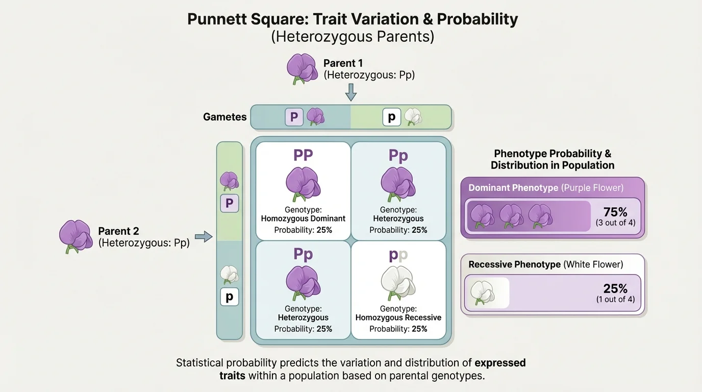
Variation also exists because biological processes involve chance. During meiosis, alleles separate into gametes. Which sperm fertilizes which egg is also random. That randomness does not mean inheritance is unpredictable; it means probability is the right tool for describing what is likely to happen across many offspring, as [Figure 2] shows for a simple dominant-recessive trait.
Genetic factors, environmental influences, and their interaction together explain why traits vary. Some traits depend mostly on inherited alleles. For example, human blood type is determined genetically. A person does not change from type \(\textrm{A}\) to type \(\textrm{O}\) because of diet or exercise.
Other traits are strongly shaped by the environment. A plant with genes for tall growth may still remain short if it lacks water, light, or nutrients. In animals, body mass can be influenced by inherited metabolism but also by food availability and physical activity. Many disease risks also reflect both inherited genes and environmental exposures.
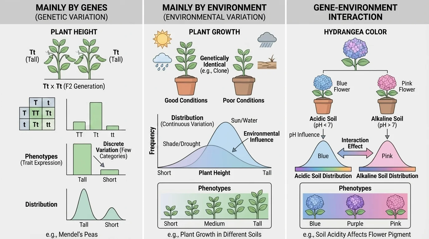
Gene-environment interaction is especially important. The same genotype can produce different phenotypes under different conditions. For example, hydrangea flower color can shift depending on soil chemistry. Similarly, identical twins may have very similar DNA, but differences in diet, stress, sun exposure, and illness can still produce observable differences.
Genes set possibilities; environments influence outcomes. In many cases, genes do not act like a fixed script. Instead, they provide a range of possible outcomes, and environmental conditions influence where within that range the organism develops. This is one reason a population often shows a spread of trait values instead of only a few exact categories.
Mutations also contribute to variation by introducing new genetic changes. Most mutations are neutral or harmful, but some create new versions of traits. Over time, mutation adds to the genetic diversity that natural selection and other evolutionary processes can act on.
When scientists predict inherited traits, they do not usually claim certainty for one individual offspring. Instead, they use probability to estimate the chance of particular outcomes. Probability tells us what is expected over many events, not what must happen in one event.
Suppose two pea plants are heterozygous for seed shape, with round \(R\) dominant over wrinkled \(r\). Each parent has a \(\dfrac{1}{2}\) chance of passing on \(R\) and a \(\dfrac{1}{2}\) chance of passing on \(r\). Combining these probabilities gives four equally likely genotype combinations: \(RR\), \(Rr\), \(Rr\), and \(rr\). That means the genotype probabilities are \(\dfrac{1}{4}RR\), \(\dfrac{1}{2}Rr\), and \(\dfrac{1}{4}rr\).
Because both \(RR\) and \(Rr\) produce round seeds, the expected phenotype probabilities are \(\dfrac{3}{4}\) round and \(\dfrac{1}{4}\) wrinkled. Written as percentages, that is \(75\%\) round and \(25\%\) wrinkled.
Worked example: predicting offspring outcomes
Two heterozygous parents with genotype \(Aa\) are crossed for a trait where \(A\) is dominant and \(a\) is recessive.
Step 1: List the possible gametes.
Each parent can pass on either \(A\) or \(a\), each with probability \(\dfrac{1}{2}\).
Step 2: Combine the possibilities.
The four equally likely outcomes are \(AA\), \(Aa\), \(Aa\), and \(aa\).
Step 3: Find genotype probabilities.
\(P(AA) = \dfrac{1}{4}\), \(P(Aa) = \dfrac{1}{2}\), and \(P(aa) = \dfrac{1}{4}\).
Step 4: Convert to phenotype probabilities.
If \(A\) is dominant, then \(AA\) and \(Aa\) show the dominant phenotype. So the dominant phenotype has probability \(\dfrac{3}{4}\), and the recessive phenotype has probability \(\dfrac{1}{4}\).
The expected ratio is \(3:1\), but actual families may differ because each birth is an independent event.
It is important not to misunderstand ratios. A \(3:1\) expected ratio does not mean that in exactly four offspring there must be three dominant and one recessive. A family of four could have four dominant phenotypes, two and two, or another combination. Probability predicts the long-run pattern across many offspring, not a guaranteed small sample.
The same probability ideas can be used for sex-linked traits, codominance, and incomplete dominance, although the phenotype patterns differ. In every case, the central idea remains the same: inheritance creates expected probabilities, and population data reveal whether observed outcomes fit those expectations closely or loosely.
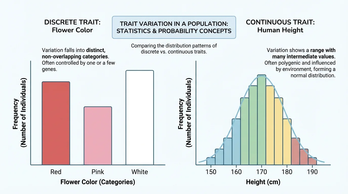
Probability helps predict possible outcomes, but statistics helps describe what is actually observed in a group, as [Figure 3] demonstrates. When biologists measure a trait in many individuals, they often calculate frequencies, proportions, percentages, averages, and spread. These numbers turn raw observations into evidence that can be compared and interpreted.
A frequency is the number of times a trait appears. A proportion compares that number to the total population. If \(18\) out of \(60\) plants have purple flowers, the proportion is \(\dfrac{18}{60} = \dfrac{3}{10} = 0.3\), and the percentage is \(30\%\).
Distributions show how trait values are spread across a population. For some traits, such as blood type, individuals fall into distinct categories. For other traits, such as height, there is a continuous range of values. Different kinds of variation are displayed with different graphs.
For numerical traits, the mean is often useful. If five plants are \(12\), \(14\), \(15\), \(17\), and \(22\) centimeters tall, then the mean height is
\[\frac{12 + 14 + 15 + 17 + 22}{5} = \frac{80}{5} = 16\]
The range describes spread. In this example, the range is \(22 - 12 = 10\) centimeters. A larger range means more variation in the measured trait.
Worked example: calculating frequency and percentage
A class studies \(40\) fast-growing bean plants. \(11\) of them have white flowers and \(29\) have purple flowers.
Step 1: State the frequency.
The frequency of white flowers is \(11\).
Step 2: Find the proportion.
\(\dfrac{11}{40} = 0.275\)
Step 3: Convert to a percentage.
\(0.275 \times 100 = 27.5\%\)
So \(27.5\%\) of the plants have white flowers.
Scientists also compare groups. For example, they might compare average heights of plants grown in sunlight and shade, or compare the frequency of a trait in two different habitats. Statistics makes those comparisons clearer and more reliable than simple guesses.
Discrete variation occurs when traits fall into separate categories with no intermediate values. Examples include blood type, attached versus unattached earlobes in simple textbook models, or flower color in some genetic crosses. These are often displayed in bar graphs because the categories are distinct.
Continuous variation occurs when traits show a range of values. Height, body mass, skin pigmentation, and leaf length are common examples. These traits are often influenced by multiple genes and by environmental factors, so the population forms a spread of values instead of neat categories. [Figure 3] shows why continuous traits are often represented by a broad curve rather than a few bars.
Human height is a classic example of a trait shaped by many genes and by environmental factors such as nutrition and health during development. That is why populations show overlapping height distributions rather than a small number of fixed height categories.
Neither type of variation is "better" or "more advanced." They simply reflect different biological mechanisms. Some traits depend strongly on one gene with a small number of possible outcomes, while others reflect many genes and environmental influence together.
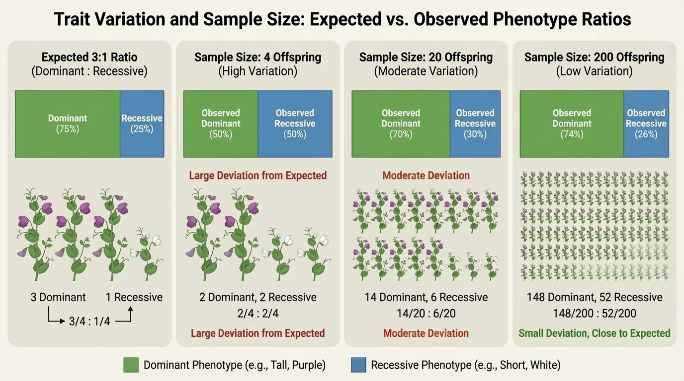
Real populations rarely fit perfectly into idealized classroom patterns. A field of pea plants may have an expected inheritance ratio, but weather, disease, soil quality, and chance can alter which plants survive long enough to be counted. Human traits are often even more complex because multiple genes and environmental factors interact over many years, as [Figure 4] makes clear.
Consider human skin pigmentation. It is influenced by several genes, and expression is also affected by sun exposure. That means a population may show a broad range of pigmentation levels, not a few sharply separated groups. Likewise, height depends on inherited growth patterns but also nutrition, illness, and hormones.
Population data reveal patterns that individuals cannot. One person's trait value tells us little about the causes of variation. When scientists measure many individuals, they can detect trends such as clustering around an average, differences between environments, or the appearance of uncommon forms of a trait.
In agriculture, breeders use these principles when selecting crops. If a farmer wants drought-tolerant plants, the farmer does not judge from one plant alone. Large samples are measured, and traits such as yield, height, or survival rate are compared statistically across many individuals and conditions.
In medicine, researchers study the distribution of traits such as blood pressure, cholesterol level, or disease risk in populations. Those traits often vary continuously. Doctors then compare an individual's measured value with the broader population distribution to decide whether it falls within a common range or an unusual one.
Many students expect inheritance problems to produce exact results, but observed data often differ from expected probabilities because of sampling variation. Random chance affects small samples strongly. The smaller the sample, the more likely it is to differ from the expected ratio.
If the expected probability of a recessive phenotype is \(\dfrac{1}{4}\), then in \(4\) offspring, seeing \(0\), \(1\), or \(2\) recessive individuals is not surprising. But in \(400\) offspring, the proportion usually comes much closer to \(\dfrac{1}{4}\). This is a major connection between probability and statistics: probability predicts what should happen in the long run, while statistics describes what actually happened in the sample.
Environmental factors can also shift observed results. Suppose a recessive plant genotype produces seedlings that are less likely to survive drought. Even if the genotype formed at the expected probability, fewer of those plants may survive to be counted. The observed phenotype distribution then reflects both inheritance and environmental filtering.
Worked example: expected and observed outcomes
A cross predicts that \(25\%\) of offspring should show a recessive trait. A class observes \(8\) recessive individuals out of \(30\) total offspring.
Step 1: Find the observed proportion.
\(\dfrac{8}{30} \approx 0.267\)
Step 2: Convert to a percentage.
\(0.267 \times 100 \approx 26.7\%\)
Step 3: Compare with the expected value.
The expected value is \(25\%\), and the observed value is about \(26.7\%\). These are close, even though they are not exactly the same.
This difference does not mean the prediction failed. It shows how real samples vary around expected probabilities.
The comparison in [Figure 4] shows why large sample sizes matter. As more individuals are measured, observed frequencies usually come closer to expected probabilities. This is why scientists prefer larger data sets when making conclusions about populations.
Science is more than naming patterns; it is explaining them with evidence. If students collect plant-height data from two groups, one with fertilizer and one without, the next step is not just to report numbers. It is to explain whether the observed difference suggests an environmental effect, a genetic effect, or both.
A strong biological explanation usually links three ideas: the source of variation, the numerical pattern, and the conclusion. For example, if the mean height of plants in rich soil is greater than the mean height in poor soil, that supports the claim that soil conditions influence the expressed trait. If flower color categories in offspring approximate a predicted ratio from inheritance, that supports a genetic explanation.
| Question | Useful tool | Example |
|---|---|---|
| What trait outcomes are likely? | Probability | \(\dfrac{3}{4}\) expected dominant phenotype |
| How common is the trait in the group? | Frequency or percentage | \(18\) of \(60\), or \(30\%\) |
| What is the typical value? | Mean | Average height of \(16\) centimeters |
| How spread out are the values? | Range and distribution | Heights from \(12\) to \(22\) centimeters |
| Does the sample match the prediction closely? | Compare observed and expected values | \(26.7\%\) observed versus \(25\%\) expected |
Table 1. Statistical and probability tools used to explain trait variation in populations.
Biologists must also avoid overclaiming. Data can support a conclusion, but one sample rarely proves a universal rule. Replication, larger sample sizes, and careful measurement make explanations stronger.
These ideas matter far beyond the classroom. In medicine, understanding trait distribution helps doctors assess risk and evaluate whether a patient's measurements are typical or unusual. In agriculture, breeders use inheritance probabilities and population data to improve crop yield, disease resistance, or drought tolerance.
Conservation biologists study trait variation to understand how populations may respond to changing environments. A population with more variation may be more likely to include individuals with traits that help survival under new conditions. This does not guarantee survival, but it increases the possibility that some individuals can reproduce successfully.
Selective breeding in animals and plants also relies on probability and statistics. Breeders track how often desired traits appear, compare distributions across generations, and decide which individuals are most likely to pass those traits on. In every case, the key idea is the same: variation is biological, but understanding it requires quantitative reasoning.
"Nothing in biology makes sense except in the light of evolution."
— Theodosius Dobzhansky
That statement becomes even more meaningful when we add statistics and probability. Evolution acts on variation, and variation can only be fully understood when we measure how traits are distributed across populations and explain why those patterns occur.