A video that goes viral, a savings account that earns interest, a car that loses value, and a medicine that slowly leaves the bloodstream may seem unrelated. But mathematically, they can all follow the same pattern: the amount changes by the same percent over each equal time interval. This kind of change is important because it may begin gradually and then become dramatic. Recognizing that pattern is one of the key ways to tell when a situation should be modeled with an exponential function instead of a linear one.
In many situations, a quantity increases or decreases by a constant amount. For example, if a water tank gains \(15\) liters every minute, then the amount changes by equal differences: \(+15, +15, +15\). That is a linear pattern.
Other situations work differently. Suppose a social media account gains \(10\%\) more followers each week than it had the week before. The increase is not a fixed number of followers each week, because \(10\%\) of a larger total is itself larger. That means the account is changing by repeated multiplication, not repeated addition. This situation can be modeled by an exponential function.
The big question is this: does the quantity change by a constant amount each interval, or by a constant percent each interval? Constant amount suggests linear behavior. Constant percent suggests exponential behavior.
Remember: A percent can be written as a decimal by dividing by \(100\). For example, \(5\% = 0.05\), \(12\% = 0.12\), and \(30\% = 0.30\). This matters because exponential growth and decay are modeled using multiplication by decimal factors.
That difference between adding and multiplying is the heart of the topic. If a quantity is repeatedly multiplied by the same factor over equal intervals, then it grows or decays at a constant percent rate.
A situation has a constant percent rate when one quantity changes by the same percentage during each equal step in another quantity, usually time. The "other quantity" might be hours, days, months, years, or even generations.
Constant percent growth means a quantity is multiplied by the same factor greater than \(1\) in each unit interval.
Constant percent decay means a quantity is multiplied by the same factor between \(0\) and \(1\) in each unit interval.
Unit interval is the equal step in the input variable, such as one hour, one month, or one year.
Growth factor is \(1 + r\), where \(r\) is the decimal form of the percent increase.
Decay factor is \(1 - r\), where \(r\) is the decimal form of the percent decrease.
If a population grows by \(3\%\) each year, then the growth factor is \(1 + 0.03 = 1.03\). Each year, you multiply by \(1.03\).
If a car loses \(18\%\) of its value each year, then the decay factor is \(1 - 0.18 = 0.82\). Each year, you multiply by \(0.82\).
The standard exponential model is
\(y = a(b)^t\)
where \(a\) is the initial value, \(b\) is the growth or decay factor, and \(t\) is the number of unit intervals.
If \(b > 1\), the quantity grows. If \(0 < b < 1\), the quantity decays.
Visual patterns help distinguish models. One of the most important graph ideas is that linear change forms a straight line because equal input changes produce equal output differences, while exponential change bends because the outputs are being repeatedly multiplied.
[Figure 1] In words, look for phrases such as "increases by \(6\%\) per year," "decreases by \(12\%\) each month," "doubles every \(5\) hours," "triples each generation," or "retains \(80\%\) of its value each year." These all describe repeated multiplication, so they point to exponential behavior.
In a table, a linear model has constant differences. An exponential model has constant ratios. For example, if the outputs are \(100, 120, 144, 172.8\), then each value is the previous one multiplied by \(1.2\), so the ratio is constant and the pattern is exponential.
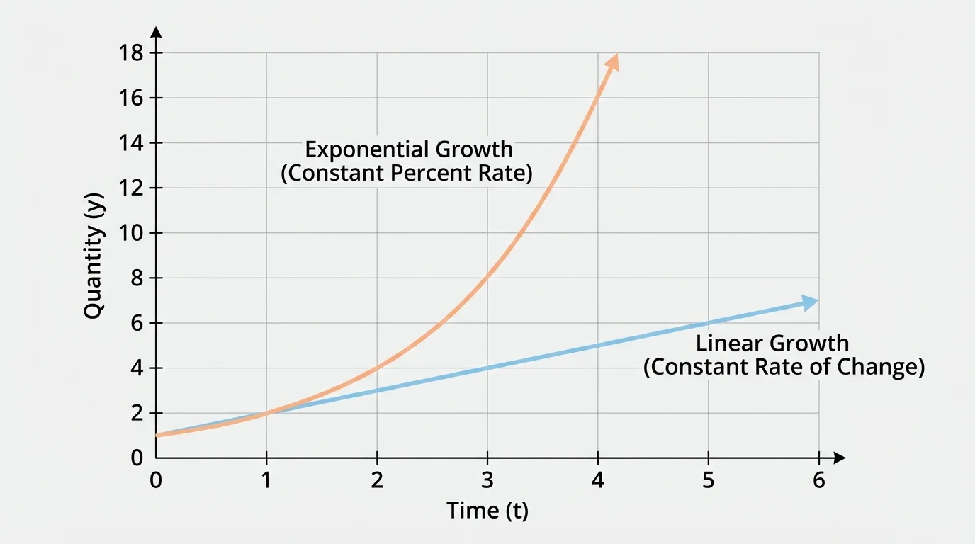
On a graph, exponential growth starts gradually and then rises more steeply. Exponential decay drops quickly at first and then levels off toward zero without usually touching it. Later, when comparing real data, this shape helps you decide whether repeated addition or repeated multiplication makes sense.
You must also pay attention to the unit interval. A quantity that changes by \(5\%\) per month is not the same as one that changes by \(5\%\) per year. The phrase "per unit interval relative to another" means the percent change is tied to equal steps in the input variable.
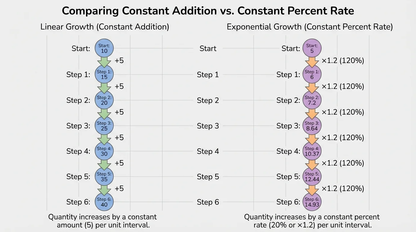
[Figure 2] shows that the comparison between additive and multiplicative change is easiest to see when values are lined up over equal intervals. Linear models keep the same difference. Exponential models keep the same ratio.
A linear model often looks like
\(y = mx + b\)
where \(m\) is the constant rate of change and \(b\) is the starting value.
An exponential model often looks like
\(y = a(b)^t\)
where \(a\) is the initial amount and \(b\) is the repeated factor.
| Feature | Linear | Exponential |
|---|---|---|
| Type of change | Constant amount | Constant percent |
| Pattern in table | Equal differences | Equal ratios |
| Equation form | \(y = mx + b\) | \(y = a(b)^t\) |
| Graph shape | Straight line | Curve |
| Typical language | "adds \(5\) each week" | "grows by \(5\%\) each week" |
Table 1. Comparison of linear and exponential models.
For instance, if a gym gains \(20\) members each month, that is linear. If the gym's membership increases by \(20\%\) each month, that is exponential. The same number, \(20\), appears in both statements, but one is an amount and the other is a percent.
This distinction matters because the outputs can become very different over time. What seems similar at first can separate quickly, especially for growth. This additive-versus-multiplicative contrast is one of the fastest recognition tools in algebra.
A quantity growing by a small percent repeatedly can eventually overtake a quantity growing by a much larger constant amount. That is one reason exponential growth plays such a major role in finance, epidemiology, and technology.
Another clue is whether the percent is based on the current amount. If the amount added or lost depends on how much is already there, then the situation is likely exponential.
A town has \(12{,}000\) people and grows by \(4\%\) each year. Recognize the type of model and write an equation for the population after \(t\) years.
Worked example
Step 1: Identify the pattern.
The population grows by a constant percent, \(4\%\), each year. Constant percent growth means the situation is exponential.
Step 2: Find the initial value and growth factor.
The initial population is \(a = 12{,}000\). The growth rate is \(r = 0.04\), so the growth factor is \(1 + 0.04 = 1.04\).
Step 3: Write the model.
Use \(P(t) = a(b)^t\): \(P(t) = 12{,}000(1.04)^t\).
The model is
\[P(t) = 12{,}000(1.04)^t\]
This model says each year's population is \(1.04\) times the previous year's population. After \(1\) year, the population is \(12{,}000(1.04) = 12{,}480\). After \(2\) years, it is \(12{,}000(1.04)^2 = 12{,}979.2\).
A car is worth $28,000 when purchased. It loses \(15\%\) of its value each year. Determine whether the model is linear or exponential, and find its value after \(3\) years.
Worked example
Step 1: Recognize the type of change.
The value decreases by a constant percent each year, so this is exponential decay.
Step 2: Find the decay factor.
The decay rate is \(0.15\), so the decay factor is \(1 - 0.15 = 0.85\).
Step 3: Write the equation.
\(V(t) = 28{,}000(0.85)^t\).
Step 4: Evaluate at \(t = 3\).
\(V(3) = 28{,}000(0.85)^3 = 28{,}000(0.614125) = 17{,}195.5\).
After \(3\) years, the car's value is approximately
\[V(3) \approx 17{,}195.5\]
So the car is worth about $17,195.50.
Notice that the car does not lose the same number of dollars each year. In the first year it loses \(0.15 \cdot 28{,}000 = 4{,}200\), but in the second year the loss is \(0.15\) of a smaller value. That changing amount is exactly why the model is exponential rather than linear.
A scientist records the number of bacteria in two dishes. Dish A has counts \(50, 100, 200, 400\) every hour. Dish B has counts \(50, 100, 150, 200\) every hour. Decide which dish shows exponential growth.
Worked example
Step 1: Check differences for each dish.
Dish A differences are \(+50, +100, +200\), which are not constant. Dish B differences are \(+50, +50, +50\), which are constant.
Step 2: Check ratios for each dish.
Dish A ratios are \(\dfrac{100}{50} = 2\), \(\dfrac{200}{100} = 2\), and \(\dfrac{400}{200} = 2\), so the ratio is constant. Dish B ratios are \(\dfrac{100}{50} = 2\), \(\dfrac{150}{100} = 1.5\), and \(\dfrac{200}{150} \approx 1.33\), so the ratio is not constant.
Step 3: Classify each pattern.
Dish A is exponential because it doubles each hour. Dish B is linear because it increases by \(50\) each hour.
Dish A shows exponential growth, and Dish B shows linear growth.
This example is important because many students first look only at whether numbers are going up. But both sets increase. The key is how they increase: by constant difference or by constant ratio.
One common mistake is treating a percent change like a constant amount. For example, "increases by \(8\%\) per year" does not mean "add \(8\) each year." It means multiply by \(1.08\) each year.
Another mistake is using the percent itself as the factor. If a quantity decays by \(30\%\), the factor is not \(0.30\). The factor is the part that remains: \(1 - 0.30 = 0.70\).
A third mistake is ignoring the interval. If a quantity grows by \(2\%\) per month, then \(t\) must count months unless the model is rewritten. Units must match.
Why repeated multiplication creates curves
When the amount of change depends on the current amount, the change itself changes over time. Large values create larger increases during growth and larger decreases during decay. That is why exponential graphs bend instead of staying straight.
It also helps to test data carefully. If the differences are almost constant but not exactly, the model may only be approximately linear. If the ratios are almost constant, the model may be approximately exponential. In real data, measurements are not always perfect, so patterns must be interpreted thoughtfully.
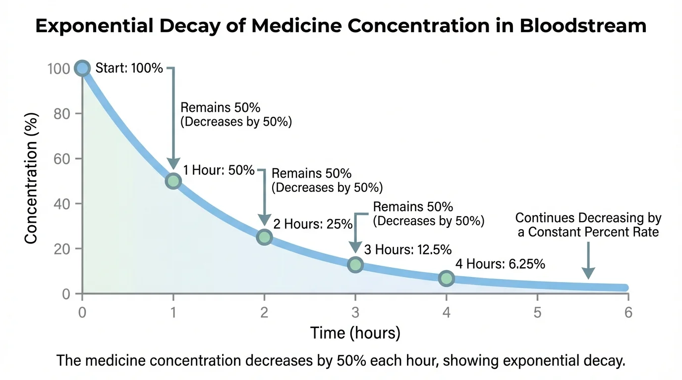
[Figure 3] Many real systems use exponential models because the change depends on the current amount. In finance, compound interest grows by a percent of the account balance. In biology, a population may grow by a percent of the current population when resources are abundant.
In medicine, drug concentration often decreases by a constant percent over equal time intervals and appears as a curve that drops quickly at first and then more slowly. This matters when doctors decide dosing schedules, because the amount removed in one hour depends on how much medicine is still present.
In technology, file compression, battery charge behavior over short intervals, and the spread of information through networks can involve repeated percentage change. In environmental science, radioactive decay and some pollutant breakdown processes also follow exponential decay.
Economics gives another useful example. Inflation may be described over time using percent increases, and investment accounts often use annual percentage growth. When such quantities are modeled over many intervals, the curved decay pattern has a curved growth pattern that can become surprisingly steep.
"Percent change sounds small until it repeats."
— A useful idea for understanding exponential models
These applications show why it is not enough to memorize formulas. You need to recognize the structure of the situation. Ask whether the amount changing each interval depends on the current amount. If it does, exponential modeling is often the right choice.
To recognize whether a quantity grows or decays by a constant percent rate per unit interval relative to another quantity, look for repeated multiplication over equal intervals. The input variable provides the intervals, and the output changes by the same percentage in each one.
If a statement says "increases by \(k\%\)," the factor is \(1 + \dfrac{k}{100}\). If it says "decreases by \(k\%\)," the factor is \(1 - \dfrac{k}{100}\). If the factor stays the same from one interval to the next, you are looking at exponential change.
Whenever you compare linear and exponential models, remember this contrast: linear means equal differences, exponential means equal ratios. That single idea explains the words, the tables, the equations, and the graphs.