A rising tide, a spinning Ferris wheel, and the changing angle of the Sun all share something unexpected: each can be modeled with trigonometric functions. That means a real-world question like "When will the water be deep enough for a boat?" can turn into an equation such as \(\sin(\theta)=0.6\). Solving that equation is not just about finding a number. It is about finding the times, angles, or positions that actually make sense in the situation.
When a periodic model is written with sine, cosine, or tangent, the unknown often appears inside the trig function. To solve for that unknown, we use inverse trigonometric functions. These functions help us reverse the effect of sine, cosine, or tangent. But because trig functions repeat, one calculator answer is often not enough. In modeling, we must find all solutions in the relevant interval and then decide which ones fit the context.
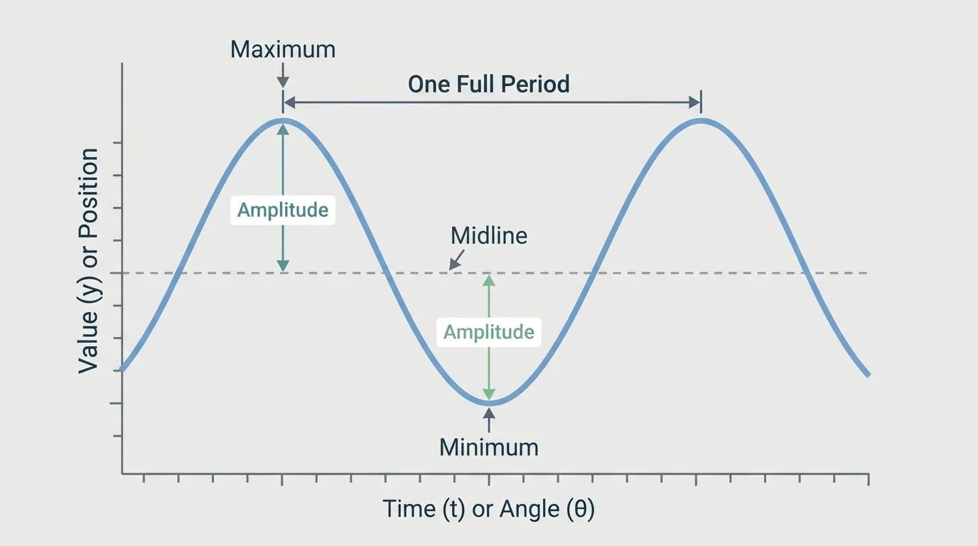
As shown in [Figure 1], a common sinusoidal model has the form \(y=A\sin(Bx-C)+D\) or \(y=A\cos(Bx-C)+D\). On a graph, the important features are the amplitude, the midline, and the period. These features tell us how high and low the values go, where the center of the motion lies, and how long one full cycle lasts.
In \(y=A\sin(Bx-C)+D\) or \(y=A\cos(Bx-C)+D\), the amplitude is \(|A|\), the midline is \(y=D\), and the period is \(\dfrac{2\pi}{|B|}\) if \(x\) is measured in radians, or \(\dfrac{360}{|B|}\) if \(x\) is measured in degrees. The quantity \(\dfrac{C}{B}\) represents a horizontal shift, often called a phase shift.
In modeling, \(x\) might represent time, angle, distance, or another changing quantity.
For example, suppose a Ferris wheel passenger's height is modeled by \(h(t)=18\cos\left(\dfrac{\pi}{10}t\right)+20\), where \(h\) is height in meters and \(t\) is time in seconds. The amplitude is \(18\), so the rider moves \(18\) meters above and below the midline. The midline is \(20\), and the period is \(\dfrac{2\pi}{\pi/10}=20\) seconds, so one complete rotation takes \(20\) seconds.
To solve equations from these models, first be sure you can identify amplitude, midline, and period. Those features help you understand what values are possible before you solve anything. For instance, if a model has amplitude \(5\) and midline \(12\), then its outputs must stay between \(7\) and \(17\).
This range check matters. If a model never goes above \(17\), then solving for when the output equals \(19\) would produce no real solution. Before using inverse trig, always ask whether the target value is even possible.
An inverse trigonometric function reverses a trigonometric function on a restricted interval. A calculator gives a single principal value, but trigonometric equations often have more than one solution because angles wrap around a circle. This is why solving in context means more than pressing a button.
The main inverse trig functions are \(\sin^{-1}(x)\), \(\cos^{-1}(x)\), and \(\tan^{-1}(x)\), often written as \(\arcsin(x)\), \(\arccos(x)\), and \(\arctan(x)\).
Their principal-value ranges are, as illustrated in [Figure 2]:
For sine, \(\arcsin(x)\) returns an angle in \(\left[-\dfrac{\pi}{2},\dfrac{\pi}{2}\right]\). For cosine, \(\arccos(x)\) returns an angle in \([0,\pi]\). For tangent, \(\arctan(x)\) returns an angle in \(\left(-\dfrac\pi2,\dfrac\pi2\right)\).
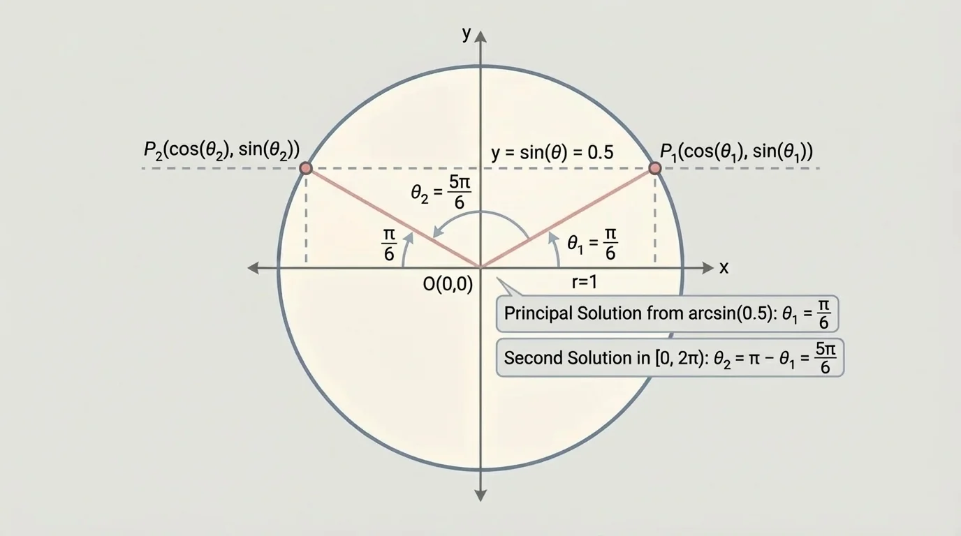
Suppose \(\sin(\theta)=0.6\). A calculator may give \(\theta\approx 36.87^\circ\) or \(\theta\approx 0.644\) radians. But in one full cycle, sine is positive in both Quadrant I and Quadrant II, so another solution is \(180^\circ-36.87^\circ=143.13^\circ\), or in radians, \(\pi-0.644\approx 2.498\).
Similarly, if \(\cos(\theta)=0.6\), cosine is positive in Quadrants I and IV. In one cycle, the solutions are \(\theta\approx 53.13^\circ\) and \(360^\circ-53.13^\circ=306.87^\circ\). If \(\tan(\theta)=0.6\), tangent repeats every \(\pi\) radians or \(180^\circ\), so solutions differ by full tangent periods.
Inverse trigonometric functions return an angle whose sine, cosine, or tangent has a given value. Because trig functions are periodic, the calculator output is usually only one angle, not every possible solution.
Principal value is the specific angle an inverse trig function is defined to return from its restricted range.
The pattern of all solutions depends on the function. For sine and cosine, you often use geometry of the unit circle or the graph to find the second solution in one cycle. For tangent, you use the repeating period to generate more solutions.
Most modeling problems follow the same path. First, write or use a trigonometric model. Next, substitute the target value and isolate the trig expression. Then apply an inverse trig function to find a principal value. After that, find all other solutions in the required interval. Finally, interpret the answers in context, including units.
Here is the general idea for a sine model. If \(A\sin(Bx-C)+D=k\), then isolate sine:
\[\sin(Bx-C)=\frac{k-D}{A}\]
Then solve for \(Bx-C\) using inverse sine and the symmetry of sine. After finding possible values of \(Bx-C\), solve each equation for \(x\).
Technology is extremely useful here. A graphing calculator or graphing app can evaluate inverse trigonometric expressions, graph both functions, and locate intersections. But technology does not replace reasoning. You still must decide whether the model uses degrees or radians and which solutions belong to the actual scenario.
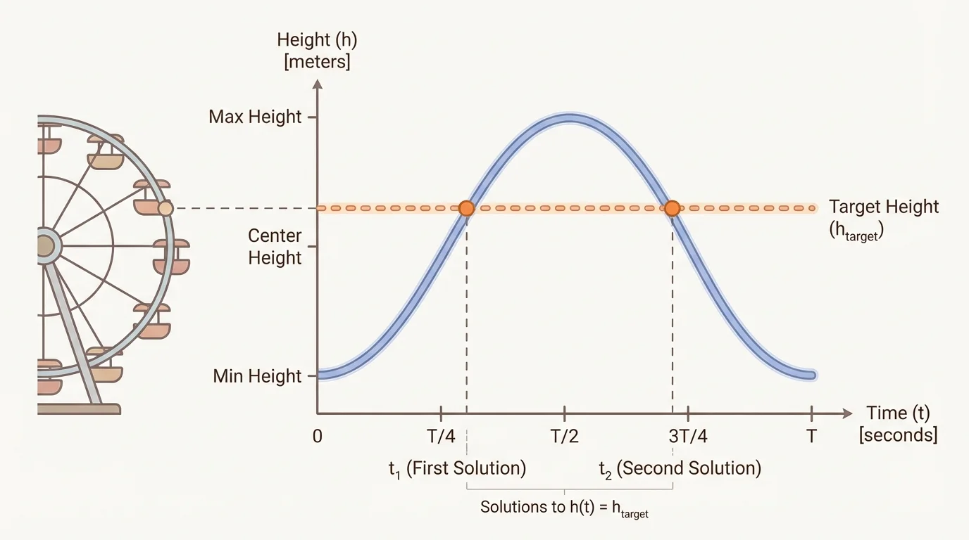
A Ferris wheel model is one of the clearest examples of trig in context, as shown in [Figure 3]. The target height appears as a horizontal line crossing the sinusoidal height graph, and the intersections represent the times we want. We solve algebraically first, then check with technology.
Worked example 1
A rider's height above the ground is modeled by \(h(t)=18\cos\left(\dfrac{\pi}{10}t\right)+20\), where \(t\) is in seconds. Find the times during one rotation when the rider is at a height of \(29\) meters.
Step 1: Set the model equal to the target height.
Substitute \(h(t)=29\): \(18\cos\left(\dfrac{\pi}{10}t\right)+20=29\).
Step 2: Isolate the cosine expression.
Subtract \(20\): \(18\cos\left(\dfrac{\pi}{10}t\right)=9\).
Divide by \(18\): \(\cos\left(\dfrac{\pi}{10}t\right)=\dfrac{1}{2}\).
Step 3: Find the angles in one cycle where cosine equals \(\dfrac{1}{2}\).
In \([0,2\pi)\), the solutions are \(\dfrac{\pi}{3}\) and \(\dfrac{5\pi}{3}\).
Step 4: Solve for time.
If \(\dfrac{\pi}{10}t=\dfrac{\pi}{3}\), then \(t=\dfrac{10}{3}\).
If \(\dfrac{\pi}{10}t=\dfrac{5\pi}{3}\), then \(t=\dfrac{50}{3}\).
The rider is at a height of \(29\) meters at
\(t=\dfrac{10}{3}\textrm{ s}\) and \(t=\dfrac{50}{3}\textrm{ s}\)
These are approximately \(3.33\) seconds and \(16.67\) seconds.
Because one rotation takes \(20\) seconds, both answers fit the interval \([0,20)\). The rider reaches \(29\) meters once while rising and once while descending. Later, if you graph the model and the line \(h=29\), the two intersections match these times.
Harbor depth changes are often modeled by sine or cosine because tides repeat regularly. In navigation, timing matters: a boat may need the water to be at least a certain depth before entering a channel.
Worked example 2
The depth of water in a harbor is modeled by \(d(t)=2.5\sin\left(\dfrac{\pi}{6}t\right)+5\), where \(d\) is depth in meters and \(t\) is time in hours after midnight. Find the times during the first \(12\) hours when the depth is \(6\) meters.
Step 1: Set the model equal to the target depth.
\(2.5\sin\left(\dfrac{\pi}{6}t\right)+5=6\)
Step 2: Isolate sine.
Subtract \(5\): \(2.5\sin\left(\dfrac{\pi}{6}t\right)=1\).
Divide by \(2.5\): \(\sin\left(\dfrac{\pi}{6}t\right)=0.4\).
Step 3: Use inverse sine to get the principal angle.
\(\arcsin(0.4)\approx 0.412\) radians.
Step 4: Find the second angle in one cycle.
Since sine is positive in Quadrants I and II, the second angle is \(\pi-0.412\approx 2.730\).
Step 5: Solve for \(t\).
If \(\dfrac{\pi}{6}t=0.412\), then \(t\approx \dfrac{6(0.412)}{\pi}\approx 0.787\).
If \(\dfrac{\pi}{6}t=2.730\), then \(t\approx \dfrac{6(2.730)}{\pi}\approx 5.214\).
During the first \(12\) hours, the depth is \(6\) meters at the following times:
\(t\approx 0.79\textrm{ h}\) and \(t\approx 5.21\textrm{ h}\)
That is about \(47\) minutes after midnight and about \(5\) hours \(13\) minutes after midnight.
Notice the interpretation step. A decimal hour like \(5.214\) hours is mathematically correct, but in navigation you might convert it to hours and minutes. The context decides how the answer should be reported.
Tidal models can be much more complicated than a single sine curve because actual tides are influenced by the Moon, the Sun, coastline shape, and local geography. Even so, a simple sinusoidal model often gives a useful first approximation.
Also notice that the model's amplitude is \(2.5\) and its midline is \(5\), so the depth ranges from \(2.5\) to \(7.5\) meters. That quick check tells us that solving for a depth like \(8\) meters would make no sense with this model.
Not every trig model is a repeating height curve. Sometimes the equation comes from geometry inside a real situation, and the inverse function gives an angle directly. This often happens with tangent.
Worked example 3
A drone is hovering \(120\) meters above level ground. An observer stands \(200\) meters horizontally from the point directly below the drone. Find the angle of elevation from the observer to the drone.
Step 1: Write a tangent equation.
In the right triangle, \(\tan(\theta)=\dfrac{120}{200}=0.6\).
Step 2: Use inverse tangent.
\(\theta=\arctan(0.6)\).
Step 3: Evaluate with technology.
In degree mode, \(\theta\approx 30.96^\circ\).
The angle of elevation is
\[\theta\approx 31.0^\circ\]
In this case, the context removes the repeating-angle issue. The angle of elevation in a right-triangle situation must lie between \(0^\circ\) and \(90^\circ\), so the principal value is the meaningful one.
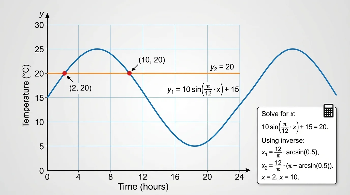
Technology helps you solve and verify equations efficiently, especially when a model has decimals or when you want to check all intersections visually, as [Figure 4] shows. A graphing calculator, Desmos, or another graphing tool can evaluate inverse trig functions and display the model over a chosen interval.
One useful method is using graph intersections. Suppose you want to solve \(18\cos\left(\dfrac{\pi}{10}t\right)+20=29\). Graph \(y=18\cos\left(\dfrac{\pi}{10}t\right)+20\) and \(y=29\). The intersection points give the solution values of \(t\). Another method is to graph the single function \(y=18\cos\left(\dfrac{\pi}{10}t\right)+20-29\) and find its zeros. A table can also help by showing when the function is close to the target value.
Be careful with radian measure and degree mode. If the model uses \(\pi\), it almost always expects radians. If the context describes rotation in degrees, degree mode may be appropriate. A wrong calculator mode can produce answers that look precise but are completely incorrect.
Technology also helps with evaluation. After you find candidate solutions, substitute them back into the model to check that they really produce the required output. In a graph, check whether the intersection lies in the interval that the situation allows. For example, a time of \(23\) seconds does not belong to a one-rotation interval of \([0,20)\).
Another strength of technology is that it shows whether there are no solutions. If a horizontal target line never crosses the graph, then the real-world event never occurs in that interval. This visual reasoning connects algebra to the context in a powerful way.
One common mistake is using only the calculator's inverse answer and stopping there. For equations involving sine and cosine, that usually misses another solution in the same cycle. Remember: inverse trig gives a principal value, not the whole story.
A second mistake is forgetting the interval. A model may repeat forever, but a question may ask for solutions during the first \(12\) hours, one day, or one rotation. The interval tells you how many valid solutions to keep.
A third mistake is ignoring the context. In a height model, negative time might not make sense. In an angle-of-elevation problem, an obtuse angle would be impossible. In a tide problem, a depth outside the model's range cannot happen. Earlier, [Figure 1] showed how the graph's amplitude and midline help predict that range before solving.
A fourth mistake is algebraic. Students sometimes apply inverse trig before isolating the trig expression. For instance, from \(2\sin(x)+3=4\), you must first get \(\sin(x)=\dfrac{1}{2}\). Only then can you use inverse sine.
Periodic models appear across science and engineering. The vertical motion of a Ferris wheel seat is sinusoidal. Tides and seasonal daylight patterns can be approximated by sinusoidal models. Alternating current in electrical systems is modeled with sine and cosine. Sound waves are often represented using trigonometric functions, and timing questions can lead to equations solved with inverse trig.
In medicine, repeated biological patterns such as breathing cycles or some forms of circadian data can be modeled periodically. In architecture and engineering, rotating parts and oscillating structures are analyzed with trig models. In astronomy, angles measured from Earth often require inverse trig functions to determine positions and elevations.
What makes these problems meaningful is interpretation. The mathematical solution is only the start. The final answer should say what the number means: a time when a rider reaches a certain height, a tide depth safe for a boat, or an angle needed to point a camera, antenna, or telescope.
"A mathematical model is useful only when you can interpret its answers in the real world."
That idea is the heart of solving trigonometric equations in context. The inverse function gives a starting point, the graph helps you find all relevant solutions, and the situation tells you which answers matter.