A stock price can rise by hundreds of dollars in a year and then drop in a week. A car can travel at different speeds during a trip. A population can grow quickly at first and then level off. In each case, one of the most useful questions is not just what the value is, but how fast it is changing. That idea is the heart of average rate of change.
When a quantity depends on another quantity, we often describe the relationship with a function. For example, the height of a ball may depend on time, the cost of electricity may depend on kilowatt-hours used, and the number of bacteria may depend on hours of growth. If we want to understand the behavior of the function, we need to know how much the output changes compared with how much the input changes.
That comparison gives a rate. In everyday life, rates appear constantly: miles per hour, dollars per item, beats per minute, degrees per hour, and gallons per minute. In functions, average rate of change tells us how quickly the output changes on average across a chosen interval.
Recall that a function assigns exactly one output value to each input value. If a function is written as \(f(x)\), then \(x\) is the input and \(f(x)\) is the output.
You may already know that slope measures how steep a line is. Average rate of change extends that same idea to any function, even when the graph is curved. Over a selected interval, we compare two points and find the slope between them.
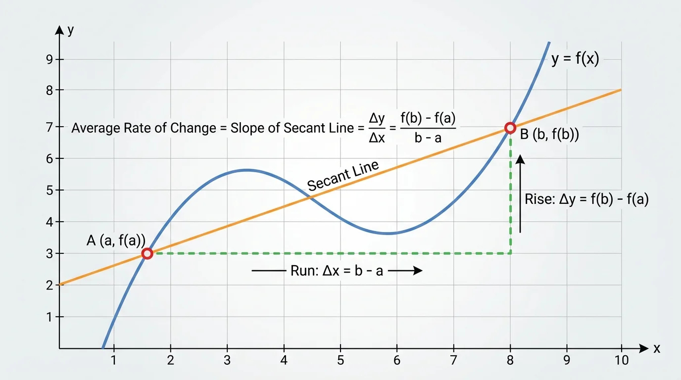
[Figure 1] The interval tells us which two input values we are comparing. If a function \(f\) is evaluated from \(x = a\) to \(x = b\), then the average rate of change over that interval is the slope between the points \((a, f(a))\) and \((b, f(b))\).
The formula is:
Average rate of change of a function \(f\) over the interval \([a,b]\) is
\[\frac{f(b)-f(a)}{b-a}\]
This compares the change in output to the change in input.
This formula looks similar to slope because it is slope. For a line, the average rate of change is the same everywhere, because the line changes at a constant rate. For a curved graph, the average rate of change depends on which interval you choose.
The numerator, \(f(b)-f(a)\), is the change in output. The denominator, \(b-a\), is the change in input. Keeping the order consistent matters. If you subtract in one order on top, you must use the same order on the bottom.
Units matter too. If height is measured in meters and time in seconds, then the average rate of change is in meters per second. If cost is measured in dollars and quantity in items, then the rate is dollars per item.
Suppose a function gives the distance a cyclist has traveled after \(t\) hours. If the average rate of change from \(t=1\) to \(t=3\) is \(18\), that means the cyclist traveled at an average of \(18\) miles per hour during that interval. It does not mean the cyclist moved at exactly \(18\) miles per hour every moment.
This distinction is important. An average rate smooths out changes that happen within the interval. Later in calculus, students study an instantaneous rate of change, which describes change at a single moment. For now, we focus on the average over an interval.
Even if two trips take the same amount of time, they can have very different average rates of change if the distances are different. Average rate is about the entire interval, not just isolated moments.
When a function is given symbolically, the process is direct: evaluate the function at the two endpoints of the interval, subtract the outputs, subtract the inputs, and divide.
If \(f(x)=3x^2-2x+1\) and the interval is \([1,4]\), then we need \(f(1)\) and \(f(4)\). Then use the formula \(\dfrac{f(4)-f(1)}{4-1}\).
Solved example 1: Symbolic function
Find the average rate of change of \(f(x)=2x^2+3\) over the interval \([1,5]\).
Step 1: Evaluate the function at the endpoints.
\(f(1)=2(1)^2+3=5\)
\(f(5)=2(5)^2+3=2(25)+3=53\)
Step 2: Compute the change in output and change in input.
Change in output: \(53-5=48\)
Change in input: \(5-1=4\)
Step 3: Divide.
\(\dfrac{48}{4}=12\)
The average rate of change is \(12\)
This means that over the interval from \(x=1\) to \(x=5\), the function's output increases by an average of \(12\) units for each increase of \(1\) unit in \(x\).
Notice that we did not need the graph to compute the answer exactly. The formula gave us the exact values at the interval endpoints.
If the function represents a real-world quantity, the answer should be interpreted in context. A rate of \(12\) might mean \(12\) feet per second, \(12\) dollars per ticket, or \(12\) degrees per hour depending on the situation.
Solved example 2: Negative average rate of change
The function \(T(t)=80-4t\) gives the temperature of a cooling liquid in degrees Celsius after \(t\) minutes. Find the average rate of change from \(t=2\) to \(t=7\).
Step 1: Evaluate the endpoints.
\(T(2)=80-4(2)=72\)
\(T(7)=80-4(7)=52\)
Step 2: Use the rate formula.
\(\dfrac{T(7)-T(2)}{7-2}=\dfrac{52-72}{5}=\dfrac{-20}{5}=-4\)
Step 3: Interpret the sign.
A negative result means the temperature is decreasing.
The average rate of change is \(-4\)
In context, the liquid cools at an average rate of \(4\) degrees Celsius per minute over that interval.
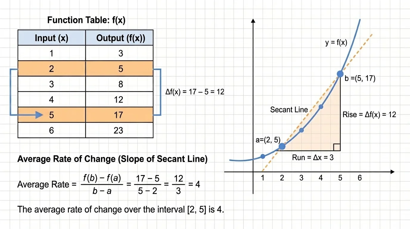
A table gives input-output pairs instead of a formula, but the idea is identical. We choose the two rows that match the interval endpoints, then compute the same quotient. The table method uses the same reasoning as the formula method, as [Figure 2] illustrates.
One common mistake is using consecutive rows even when the question asks for a wider interval. Always check the actual input values named in the problem.
For example, suppose a table gives the value of a function \(g(x)\):
| \(x\) | \(g(x)\) |
|---|---|
| \(0\) | \(4\) |
| \(2\) | \(10\) |
| \(5\) | \(19\) |
| \(8\) | \(31\) |
Table 1. Input and output values for the function \(g(x)\).
If we want the average rate of change on \([2,8]\), we use only \((2,10)\) and \((8,31)\). The middle row at \(x=5\) is not needed.
Now compute: \(\dfrac{31-10}{8-2}=\dfrac{21}{6}=3.5\). So the average rate of change is \(3.5\).
Solved example 3: Table of values
The table shows the height \(h\) of a plant in centimeters after \(d\) days.
| \(d\) | \(h(d)\) |
|---|---|
| \(1\) | \(12\) |
| \(4\) | \(18\) |
| \(6\) | \(23\) |
| \(10\) | \(35\) |
Table 2. Plant height as a function of time in days.
Find the average rate of change from day \(4\) to day \(10\).
Step 1: Identify the endpoint values.
\(h(4)=18\) and \(h(10)=35\)
Step 2: Find the changes.
Change in height: \(35-18=17\)
Change in days: \(10-4=6\)
Step 3: Divide.
\(\dfrac{17}{6}\approx 2.83\)
The average rate of change is \[\frac{17}{6}\approx 2.83\]
Interpretation: over that interval, the plant grows at an average of about \(2.83\) centimeters per day.
As with formulas, the units come from output units divided by input units. Here that is centimeters per day.
Later, when comparing intervals, you may find that the average rate changes from one interval to another. That signals that the function is not linear.
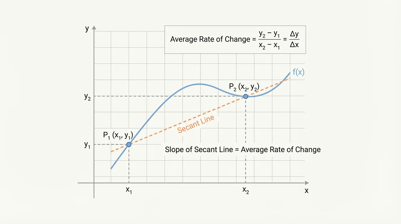
Graphs are powerful because they let you see overall behavior, but they often require estimation instead of exact computation. To estimate average rate of change from a graph, choose the two x-values of the interval, read the corresponding y-values as carefully as possible, and use the slope formula. This visual method is shown in [Figure 3].
Suppose a graph shows the height of a drone over time. If the interval is from \(t=2\) to \(t=6\), locate those x-values on the horizontal axis, move up or down to the graph, and estimate the y-values from the vertical axis.
If the graph appears to pass near \((2,15)\) and \((6,27)\), then the estimated average rate of change is \(\dfrac{27-15}{6-2}=\dfrac{12}{4}=3\). The drone's height increases at about \(3\) units of height per unit of time on that interval.
Because graph reading is approximate, small differences are normal. If one student estimates \((2,14.8)\) and another estimates \((2,15.2)\), their answers may differ slightly. What matters is reasonable reading and correct method.
When a graph is curved, the secant line between two points gives the average rate over the whole interval. That is why the graph in [Figure 1] remains useful even when the function is not a line.
Average rate from a graph is a slope estimate
On a graph, average rate of change is estimated by finding the slope of a secant line. A secant line crosses the graph at two points, one at each endpoint of the interval. Its steepness tells how the function changes on average between those points.
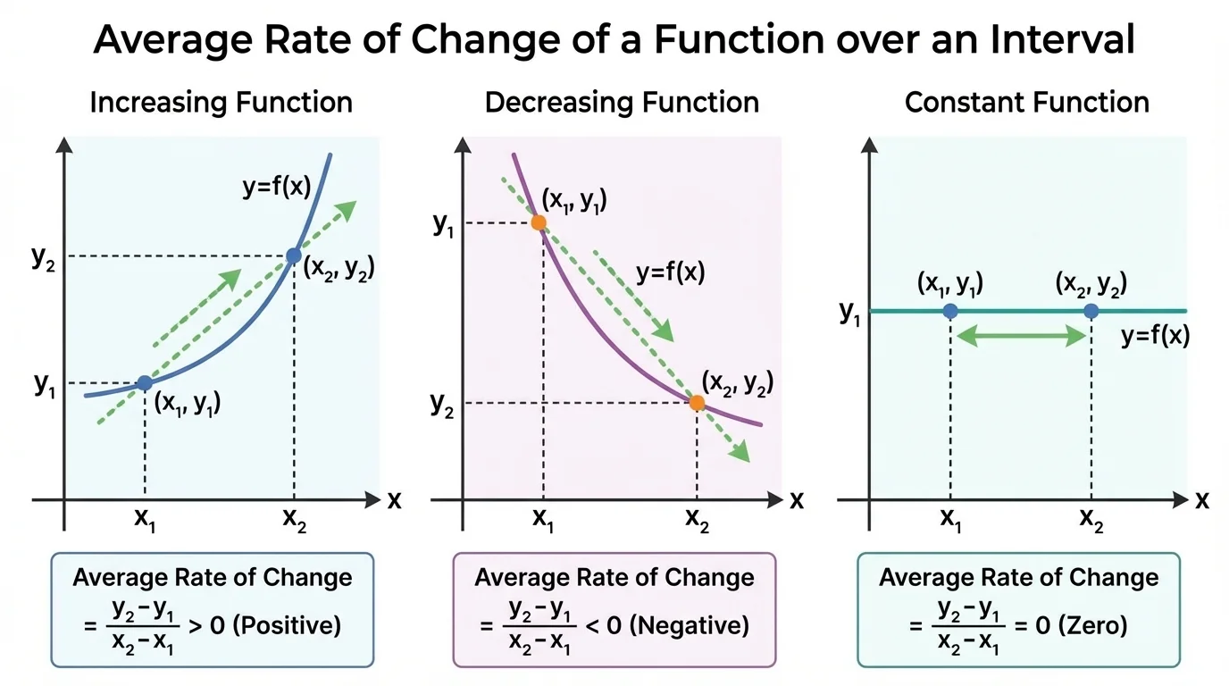
[Figure 4] The sign of the rate tells an important story. A positive rate means the function increases over the interval. A negative rate means it decreases. A rate of zero means the output has the same value at both endpoints.
If a business's profit changes from \(\$5{,}000\) to \(\$8{,}000\) over \(3\) months, the average rate of change is positive. If a car's fuel amount changes from \(12\) gallons to \(4\) gallons over \(2\) hours, the rate is negative. If a hiker starts and ends the interval at the same elevation, the average rate over that interval is zero.
The size of the rate matters too. A larger positive value means a faster increase. A more negative value means a faster decrease. A rate close to zero means little overall change.
Also, a function can have different average rates on different intervals. For instance, a runner may speed up early in a race and slow down later. Looking at several intervals helps describe that changing behavior more accurately.
One frequent error is mixing subtraction orders. If you compute \(f(b)-f(a)\), then the denominator must be \(b-a\). If you reverse the top to \(f(a)-f(b)\), then you must reverse the bottom to \(a-b\). Otherwise, the sign will be wrong.
Another mistake is using the wrong points from a table or graph. The interval determines the endpoints. If the interval is \([3,9]\), then use values at \(x=3\) and \(x=9\), not nearby values unless you are estimating from a graph and exact points are unavailable.
Solved example 4: Catching an order mistake
A student finds the average rate of change of \(f(x)=x^2\) on \([2,6]\) and writes \(\dfrac{36-4}{2-6}=\dfrac{32}{-4}=-8\). What went wrong?
Step 1: Check the endpoint outputs.
\(f(2)=4\) and \(f(6)=36\). These are correct.
Step 2: Check the subtraction order.
The numerator uses \(f(6)-f(2)=36-4\), so the denominator must use \(6-2\), not \(2-6\).
Step 3: Recalculate correctly.
\(\dfrac{36-4}{6-2}=\dfrac{32}{4}=8\)
The correct average rate of change is \(8\)
A third mistake is forgetting units. A numeric answer without context can be incomplete. In science and real-life applications, units often carry the meaning of the entire rate.
Finally, do not confuse average rate of change with the function value itself. If the function output is \(50\), that does not mean the rate is \(50\). The rate compares two outputs over two inputs.
Average rate of change appears in medicine, economics, environmental science, and engineering. Doctors may track the change in a patient's heart rate over time. Economists may study how unemployment changes over a quarter. Engineers may analyze how temperature changes in a machine as it runs.
In environmental science, suppose the amount of water in a reservoir is modeled by a function of time. The average rate of change over a week tells whether the reservoir is filling or draining overall. A positive rate means net gain; a negative rate means net loss.
In business, a company may compare revenue over two months. If revenue rises from \(\$20{,}000\) to \(\$26{,}000\) over \(2\) months, the average rate of change is \(\dfrac{26{,}000-20{,}000}{2}=3{,}000\) dollars per month. That helps describe growth more clearly than just saying the revenue changed.
Solved example 5: Real-world interpretation
A car rental company models the total cost \(C(d)\) in dollars for renting a car for \(d\) days. Suppose \(C(2)=98\) and \(C(6)=250\). Find and interpret the average rate of change from \(d=2\) to \(d=6\).
Step 1: Compute the change in cost.
\(250-98=152\)
Step 2: Compute the change in days.
\(6-2=4\)
Step 3: Divide and interpret.
\(\dfrac{152}{4}=38\)
The average rate of change is \(38\)
Interpretation: over that interval, the rental cost increases by an average of \(\$38\) per day.
As seen earlier in [Figure 3], graphs are especially useful when exact equations are not available. In real data, that happens often: scientists and analysts may only have measurements and plots.
No matter how a function is presented, the underlying idea stays the same. A formula gives exact values through substitution. A table gives selected values directly. A graph shows trends visually and supports estimation. The same core quantity is always being computed:
change in output divided by change in input.
| Representation | What you use | Main challenge |
|---|---|---|
| Formula | Evaluate \(f(a)\) and \(f(b)\) | Correct substitution |
| Table | Read endpoint rows | Choosing correct interval endpoints |
| Graph | Estimate endpoint coordinates | Reading values accurately |
Table 3. Comparison of how average rate of change is found from different representations.
Across all three representations, the sign and units still tell the story of how the function changes in context. That is why this topic is so useful in applications.