A rideshare app charges a base fee, then adds the same amount for every mile. A streaming service adds the same monthly cost to your total spending. A runner moving at a steady speed covers equal distances in equal amounts of time. These situations may look different, but they share a powerful mathematical idea: one quantity changes at a constant rate relative to another. Recognizing that pattern helps you decide when a situation can be modeled by a line instead of something more complicated.
When we say one quantity changes at a constant rate per unit interval relative to another, we mean that for every increase of one unit in the input quantity, the output quantity changes by the same amount every time. If the input is time, then each extra hour, minute, or day produces the same increase or decrease in the other quantity.
Constant rate of change means that equal changes in one variable produce equal changes in another variable.
Unit interval means an increase of exactly one unit in the input variable, such as from \(2\) to \(3\), or from \(10\) to \(11\).
Rate of change compares how much one quantity changes relative to a change in another quantity.
If a plant grows \(2\) centimeters every week, then its height changes at a constant rate of \(2\) centimeters per week. If your savings account balance goes up by $15 every week because you deposit the same amount, that balance changes at a constant rate of $15 per week.
The word linear function is closely connected to this idea. A situation with a constant additive change is often modeled by a linear function. That means the graph is a straight line, and the equation can usually be written in the form \(y = mx + b\), where \(m\) is the constant rate and \(b\) is the starting value.
Not every changing quantity has a constant rate. Some situations speed up, slow down, or change by percentages instead of by equal amounts. A constant rate means add the same amount each time. If the amount being added changes, then the rate is not constant.
For example, suppose a gym membership costs $25 to join and then $10 per visit. After each visit, the total cost increases by exactly $10. That is a constant rate, so it is linear. But if a population grows by \(5\%\) each year, the amount added each year gets larger over time. That is not a constant additive rate, so it is not linear.
Equal differences versus equal factors
Linear growth is based on equal differences. If the output values go \(5, 8, 11, 14\), the difference is always \(+3\). Exponential growth is based on equal factors. If the values go \(5, 10, 20, 40\), each value is multiplied by \(2\). Equal differences signal a linear model; equal factors signal an exponential model.
This distinction matters because two situations can both be increasing, but only one may have a constant rate per unit interval. Mathematics is not just about noticing growth; it is about noticing how the growth happens.
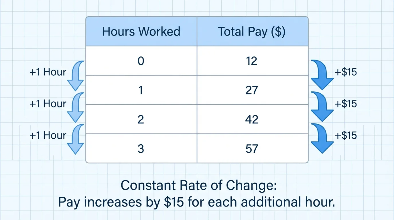
You can detect a constant rate of change in several representations. In a table, equal jumps in the input should produce equal changes in the output, as shown in [Figure 1]. If \(x\) increases by \(1\) each time, then the differences in \(y\) should all match.
Suppose a table shows the total amount earned after working different numbers of hours:
| Hours worked \((x)\) | Total pay \((y)\) |
|---|---|
| \(0\) | \(12\) |
| \(1\) | \(27\) |
| \(2\) | \(42\) |
| \(3\) | \(57\) |
Table 1. Hours worked and total pay for a job with a fixed starting amount and constant hourly earnings.
The pay increases by \(15\) each hour: \(27 - 12 = 15\), \(42 - 27 = 15\), and \(57 - 42 = 15\). Since the change is always \(15\) for each increase of \(1\) hour, the rate is constant.
In a graph, a constant rate appears as a straight line. If the graph curves, bends, or becomes steeper and steeper, the rate is changing. A straight line means that the steepness stays the same all along the graph.
In words, listen for phrases such as each hour adds, per mile, for every, or increases by the same amount each time. These often signal a constant rate. On the other hand, phrases such as doubles every year, grows by \(8\%\), or triples every decade usually signal exponential change instead.
In an equation, a linear model has the form \(y = mx + b\). The coefficient \(m\) tells how much \(y\) changes when \(x\) increases by \(1\). If an equation includes exponents on the variable, such as \(y = 3(2)^x\), then the situation is not linear.
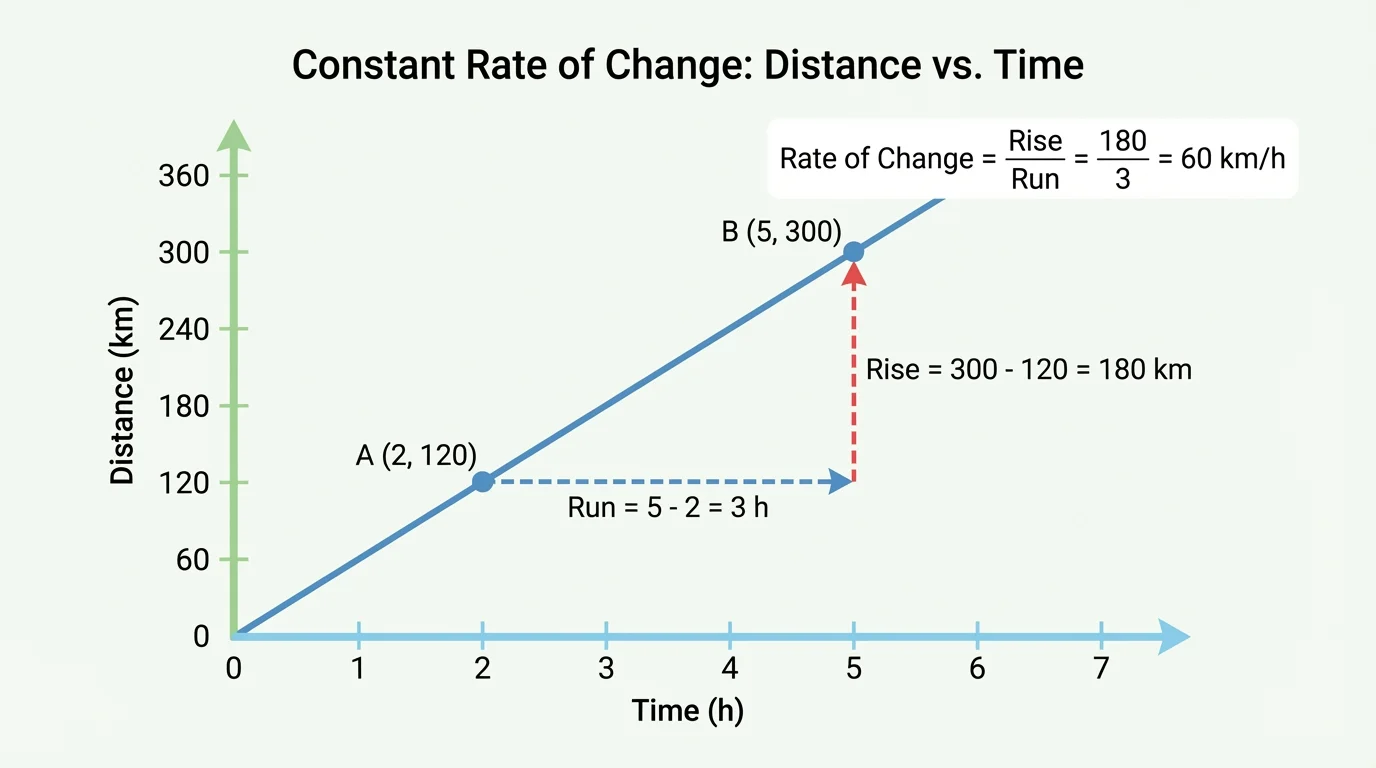
The slope of a line measures its constant rate of change. It tells how much the output changes compared with the input, and its visual meaning becomes clear in [Figure 2], where the rise and run stay proportional along the same line.
If you know two points \((x_1, y_1)\) and \((x_2, y_2)\), the slope is found by dividing the change in \(y\) by the change in \(x\):
\[m = \frac{y_2 - y_1}{x_2 - x_1}\]
If the slope is positive, the line rises from left to right, meaning the output increases as the input increases. If the slope is negative, the line falls from left to right, meaning the output decreases. If the slope is \(0\), the output stays constant no matter what happens to the input.
For a linear equation \(y = mx + b\), the number \(m\) is the constant rate of change. For example, in \(y = 4x + 7\), the rate is \(4\). Every time \(x\) increases by \(1\), \(y\) increases by \(4\).
The number \(b\) is different. It is the starting value, also called the \(y\)-intercept. Students often confuse the rate with the starting value, so it is important to separate them: \(m\) tells how fast the quantity changes, while \(b\) tells where it starts.
Recognizing a constant rate gets easier when you work through different forms of information.
Worked example 1: Identifying constant rate from a table
A table shows the temperature of a cooling object over time.
| Time \((x)\) in minutes | Temperature \((y)\) in \(^\circ\textrm{C}\) |
|---|---|
| \(0\) | \(90\) |
| \(1\) | \(86\) |
| \(2\) | \(82\) |
| \(3\) | \(78\) |
Table 2. Time and temperature values for a cooling object.
Step 1: Compare the changes in the input.
The time increases by \(1\) minute each row.
Step 2: Compare the changes in the output.
\(86 - 90 = -4\), \(82 - 86 = -4\), and \(78 - 82 = -4\).
Step 3: Interpret the result.
The temperature decreases by \(4\) degrees each minute, so the rate of change is constant.
The situation is linear, with constant rate \(-4\) degrees per minute.
Notice that the output is decreasing, but it is still linear because the decrease happens by the same amount every time.
Worked example 2: Finding the rate from an equation
Determine whether the equation \(y = -3x + 18\) represents a constant rate of change, and identify the rate.
Step 1: Recognize the form.
The equation is in the form \(y = mx + b\).
Step 2: Identify \(m\).
Here, \(m = -3\).
Step 3: Interpret the meaning.
For every increase of \(1\) in \(x\), the value of \(y\) decreases by \(3\).
Yes, the equation represents a constant rate of change, and the rate is \(-3\).
This is one of the fastest ways to recognize a constant rate: if the equation is linear, the rate is the coefficient of \(x\).
Worked example 3: Using two points to test for constant rate
A car travels so that its distance from home is represented by the points \((2, 110)\) and \((5, 170)\), where \(x\) is time in hours and \(y\) is distance in miles. Find the rate of change.
Step 1: Use the slope formula.
\(m = \dfrac{y_2 - y_1}{x_2 - x_1}\)
Step 2: Substitute the coordinates.
\(m = \dfrac{170 - 110}{5 - 2} = \dfrac{60}{3}\)
Step 3: Simplify.
\(m = 20\)
The distance changes at a constant rate of \(20\) miles per hour.
Because the relationship between time and distance has a constant slope, it can be modeled with a linear function if the motion remains steady.
Worked example 4: Deciding between linear and non-linear
Which situation has a constant rate per unit interval?
Situation A: A video game score increases by \(250\) points after each completed level.
Situation B: The number of views on a video increases by \(20\%\) each day.
Step 1: Look for equal differences or equal factors.
Situation A adds \(250\) each level. Situation B multiplies by \(1.20\) each day.
Step 2: Identify the pattern.
Equal differences mean a constant additive rate. Equal factors mean exponential change.
Step 3: Decide.
Situation A has a constant rate of change. Situation B does not have a constant additive rate.
Only Situation A is linear.
One of the most important skills in algebra is deciding whether a context is linear or exponential. The visual contrast is striking in [Figure 3]: linear growth forms a straight line, while exponential growth curves because the rate itself changes.
Suppose a bank account receives a deposit of $50 every month. The balance rises by the same amount each month, so the pattern is linear. But if money grows by interest at \(4\%\) per year, the amount added each year depends on the current balance. The larger the balance becomes, the larger the yearly increase becomes. That changing increase means the rate is not constant.
Here is a quick comparison:
| Feature | Linear | Exponential |
|---|---|---|
| Type of change | Equal differences | Equal factors |
| Rate per unit interval | Constant | Not constant in an additive sense |
| Typical equation | \(y = mx + b\) | \(y = ab^x\) |
| Graph shape | Straight line | Curve |
Table 3. Comparison of linear and exponential patterns.
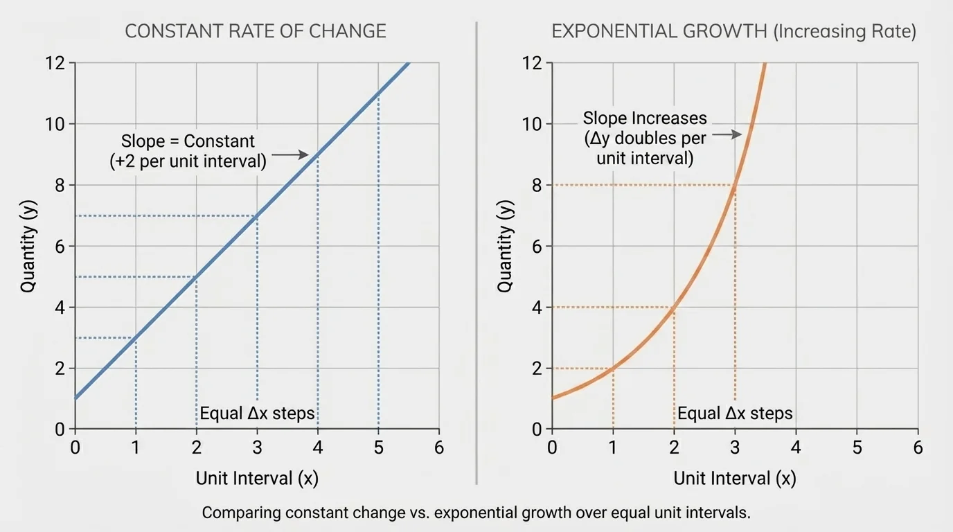
A useful test is this: ask, "When the input increases by \(1\), does the output change by the same amount?" If so, the situation is linear. If the output changes by the same factor or percentage instead, then it is exponential.
Earlier, [Figure 1] showed how equal differences in a table reveal linear behavior. That same idea explains why exponential tables fail the constant-difference test even when the numbers increase smoothly.
Constant rates appear in many serious, real-world settings. In manufacturing, a machine that produces \(120\) parts per hour at a steady pace has a linear output model. In transportation, a car traveling at a constant speed covers equal distances in equal times. In business, a company with a fixed startup fee plus a constant cost per item often uses a linear pricing model.
Phone plans are another example. A plan might charge $35 per month plus $5 for each extra gigabyte of data. If \(x\) is the number of extra gigabytes, the total monthly cost is modeled by \(y = 5x + 35\). The rate of change is \(5\), meaning each extra gigabyte adds $5.
In physics, many introductory models assume constant speed or constant acceleration over short periods. When speed is constant, distance depends linearly on time. If an object moves at \(12\) meters per second, then after \(t\) seconds, the distance is \(d = 12t\). The slope \(12\) represents the constant rate, and the line passes through the origin because the starting distance is \(0\).
The same rise-over-run idea from [Figure 2] helps interpret these contexts. A steeper line means a larger rate, whether that means faster travel, higher hourly earnings, or greater fuel consumption per mile.
Many professional decisions depend on recognizing constant rates quickly. Engineers compare rates of material use, economists track linear cost models over short ranges, and scientists often begin with linear approximations before studying more complex behavior.
Even when the real world becomes more complicated, recognizing a constant rate is often the first step in building a useful mathematical model.
A common mistake is looking only at whether values are increasing and then assuming the rate is constant. Increase alone is not enough. The increase must be by the same amount each unit interval.
Another mistake happens when the intervals in the input are not equal. If the input changes from \(1\) to \(3\), then from \(3\) to \(4\), you cannot compare raw output differences directly. You must compare the change per unit. For example, if \(y\) changes by \(10\) when \(x\) changes by \(2\), the rate is \(\dfrac{10}{2} = 5\) per unit.
Students also sometimes confuse a constant rate with a constant starting value. In \(y = 7x + 2\), the constant rate is \(7\), not \(2\). The number \(2\) tells the value of \(y\) when \(x = 0\).
Finally, do not confuse a straight-line pattern in a small part of a graph with a truly linear relationship over the full domain. Some real situations are only approximately linear for short intervals. Good modeling requires paying attention to context.
"Equal changes in equal intervals"
— A simple test for recognizing linear change
When you learn to spot constant rates, you are doing more than identifying a formula. You are recognizing structure in the world: when costs accumulate steadily, when motion remains uniform, when a graph stays straight, and when a table's differences remain constant. That skill is one of the foundations of algebraic modeling.