A basketball player scores \(12\) points in one game and \(28\) in the next. Another player scores \(20\) points in both games. Both players average \(20\) points, but do they really perform the same way? That question shows why statistics is so useful. A set of numbers can often be described with just one or two important summaries, but choosing the right summaries matters.
When people collect numbers such as test scores, daily temperatures, heights of plants, or the number of minutes it takes to get to school, they often want a quick way to describe the whole set. A data set is a collection of values. A single number can help us describe the data set without listing every value again.
A measure of center tells what value is typical or in the middle of the data in some way. But center alone does not tell the whole story. A measure of variation tells how much the values differ from one another. In other words, center tells where the data are located, and variation tells how spread out the data are.
Measure of center is a number used to describe a typical value of a data set. Common measures of center are the mean, median, and mode.
Measure of variation is a number used to describe how much the values in a data set spread out. A common measure of variation in grade \(6\) is the range.
If two classes both have an average quiz score of \(80\), that does not mean the classes performed in the same way. One class might have scores very close to \(80\), while the other class might have some very high scores and some very low scores. Looking at both center and variation gives a much better picture.
There are several ways to describe the center of a data set. Each one uses the values in a different way.
The mean is what many people call the average. To find the mean, add all the values and divide by the number of values. If the data set is \(4, 6, 8\), then the mean is
\[\frac{4+6+8}{3}=\frac{18}{3}=6\]
The median is the middle value when the data are listed in order from least to greatest. For example, in the data set \(3, 5, 7, 9, 12\), the median is \(7\) because it is the middle value.
The mode is the value that appears most often. In the data set \(2, 4, 4, 5, 7\), the mode is \(4\).
These measures of center do not always give the same number. That is normal. Each measure highlights a different feature of the data. The mean uses every value. The median depends on the order of the values and the middle position. The mode focuses on the most frequent value.
To find the median correctly, always put the numbers in order first. To find the mean correctly, include every value in the sum and divide by the total number of values.
Sometimes one measure of center is more helpful than another. If the data have one unusual value that is much larger or smaller than the rest, the mean can change a lot, while the median may stay closer to what most of the data look like.
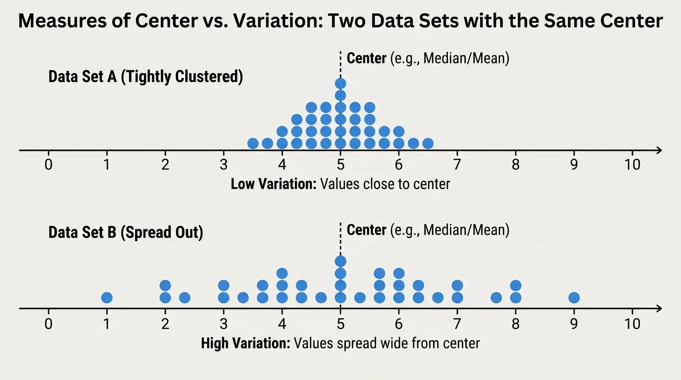
Two data sets can have the same center but very different spread, as [Figure 1] shows. That spread is called variation. If the values stay close together, the variation is small. If the values are far apart, the variation is large.
A simple way to measure variation is the range. The range is the difference between the greatest value and the least value.
For example, in the data set \(5, 6, 7, 8, 9\), the range is
\(9-5=4\)
In the data set \(1, 3, 7, 11, 13\), the range is
\(13-1=12\)
Both sets have a center near \(7\), but the second set is much more spread out. That means it has greater variation. Looking only at the center would hide that difference.
Another useful way to think about variation is to ask, "How far are the values from the center?" If most values are near the center, variation is low. If many values are far from the center, variation is high.
This is why statisticians do not stop after finding just one average. A good summary usually includes both a measure of center and a measure of variation.
Let us compare these two data sets:
Set A: \(4, 5, 6, 7, 8\)
Set B: \(2, 4, 6, 8, 10\)
Worked example
Step 1: Find the mean of Set A.
Add the values: \(4+5+6+7+8=30\). There are \(5\) values, so the mean is \(30 \div 5 = 6\).
Step 2: Find the mean of Set B.
Add the values: \(2+4+6+8+10=30\). There are \(5\) values, so the mean is also \(30 \div 5 = 6\).
Step 3: Find the range of Set A.
The greatest value is \(8\) and the least value is \(4\), so the range is \(8-4=4\).
Step 4: Find the range of Set B.
The greatest value is \(10\) and the least value is \(2\), so the range is \(10-2=8\).
Both sets have mean \(6\), but Set B has a larger range. So Set B has greater variation.
This example is important because it shows that the same center does not mean the same data. Set A is packed more closely around \(6\), while Set B is more spread out. That is the exact job of a measure of variation: it tells us something center cannot tell us.
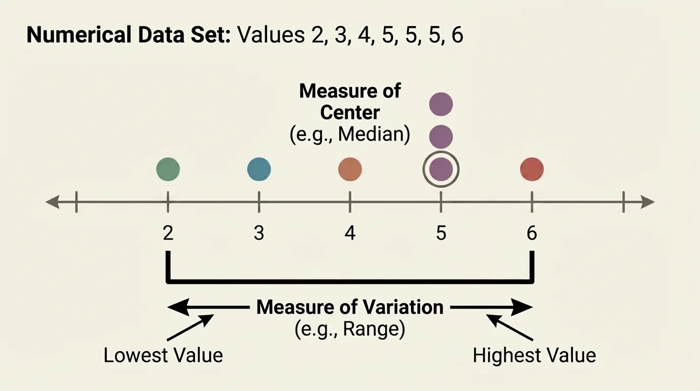
Ordering data helps reveal the middle value and the spread. [Figure 2] illustrates this idea. Consider the data set showing the number of books read by \(7\) students in a month: \(2, 5, 3, 4, 5, 6, 5\).
Worked example
Step 1: Order the data.
The ordered data set is \(2, 3, 4, 5, 5, 5, 6\).
Step 2: Find the mean.
Add the values: \(2+3+4+5+5+5+6=30\). There are \(7\) values, so the mean is \(30 \div 7\).
\[\frac{30}{7}=4\frac{2}{7}\approx 4.29\]
Step 3: Find the median.
There are \(7\) values, so the middle is the \(4\)th value. The median is \(5\).
Step 4: Find the mode.
The value \(5\) appears most often, so the mode is \(5\).
Step 5: Find the range.
The greatest value is \(6\) and the least value is \(2\), so the range is \(6-2=4\).
The data set can be summarized by saying its center is around \(5\), and its range is \(4\).
Notice that the mean is about \(4.29\), while the median and mode are both \(5\). This tells us that different measures of center can describe the same data in slightly different ways. None of them is automatically wrong. We choose the one that best helps us understand the situation.
When the data are placed in order on a number line, it becomes easier to see the median as the middle position and the range as the distance from the smallest to the largest value.
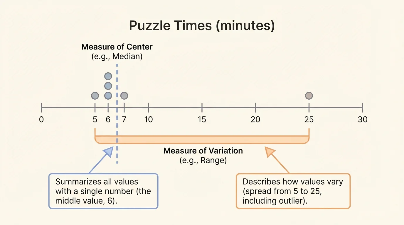
One unusual value, called an outlier, can pull the mean away from the rest of the data. Suppose five students take \(5\) minutes, \(6\) minutes, \(6\) minutes, \(7\) minutes, and \(25\) minutes to finish a puzzle.
[Figure 3] Most of the times are between \(5\) and \(7\) minutes, but one time is \(25\) minutes. That value is much larger than the others, so it is an outlier.
Worked example
Step 1: Find the mean.
Add the values: \(5+6+6+7+25=49\). Divide by \(5\): \(49 \div 5 = 9.8\).
Step 2: Find the median.
The ordered data are already \(5, 6, 6, 7, 25\). The middle value is \(6\), so the median is \(6\).
Step 3: Compare the summaries.
The mean is \(9.8\), but most students actually finished in about \(6\) minutes. The median \(6\) describes the typical time better than the mean in this case.
This data set shows why we should think about the shape of the data, not just compute numbers.
The range here is \(25-5=20\), which is large because of the outlier. This also shows that one unusual value can affect variation strongly. When you compare data sets, look carefully for values that are far away from the rest.
Weather reports often use averages, but meteorologists also care about variation. A week with temperatures \(21, 21, 22, 21, 22\) feels more steady than a week with \(10, 18, 22, 27, 30\), even if the average temperature is similar.
Measures of center and variation appear all around you. Sports announcers talk about average points per game, teachers look at class quiz averages, and scientists track average rainfall. But in each case, variation matters too.
Suppose two runners both average \(8\) minutes for a mile over \(4\) practices. Runner A has times \(8, 8, 8, 8\). Runner B has times \(6, 7, 9, 10\). The mean for both is
\[\frac{32}{4}=8\]
Yet Runner A is very consistent, while Runner B is less consistent. Runner A has range \(8-8=0\), and Runner B has range \(10-6=4\). A coach would learn more by knowing both the center and the variation.
Travel time is another example. If your trip to school usually takes about \(15\) minutes, that is a measure of center. But if some days it takes \(8\) minutes and other days \(25\) minutes, then the variation is large. That means the trip is not very predictable.
When comparing two groups, ask two questions. First, which group has the higher center? Second, which group has the greater variation?
For example, Class A has scores \(70, 72, 74, 76, 78\). Class B has scores \(60, 70, 74, 78, 88\). Both classes have mean
\[\frac{370}{5}=74\]
But the ranges are different. Class A has range \(78-70=8\). Class B has range \(88-60=28\). So both classes have the same mean, but Class B's scores are much more spread out. This is similar to what we saw earlier in [Figure 1], where equal centers still hid very different spreads.
If a principal wants to know which class had more consistent results, the variation matters more. If the principal wants a quick idea of the overall performance level, the center matters more. Often both are needed.
Why center and variation belong together
A measure of center gives one number to represent the data set, but no single center can describe every feature of the data. A measure of variation adds a second piece of information: whether the values stay close to that center or scatter far away from it. Together, these summaries create a clearer picture.
You can think of center as answering, "Where are the data?" and variation as answering, "How spread out are the data?" Those two questions are the heart of understanding statistical variability.
One common mistake is thinking that if two data sets have the same mean, they must be alike. The examples in this lesson show that this is not true.
Another mistake is forgetting to order the data before finding the median. Without ordering, the middle position cannot be found correctly.
A third mistake is ignoring an outlier. As we saw in [Figure 3], one unusual value can change the mean and range a lot. That can make a data set seem more spread out or shift the average away from what most values show.
Students also sometimes mix up mode and median. Remember: mode is the most frequent value, while median is the middle value in order.
| Measure | What it tells you | How to find it |
|---|---|---|
| Mean | A balance point or average of all values | Add all values and divide by the number of values |
| Median | The middle value | Put values in order and find the middle |
| Mode | The most common value | Find the value that appears most often |
| Range | How far apart the smallest and largest values are | Subtract least value from greatest value |
Table 1. A comparison of common measures of center and variation for grade 6 statistics.
The more you work with data, the more natural these summaries become. What matters most is understanding what the numbers mean. A center without variation is incomplete, and variation without center does not tell you what value is typical. Statistics becomes powerful when both ideas are used together.