Weather forecasts, sports statistics, and even video game mechanics all depend on the same big idea: chance has patterns. A single result can surprise you, but when a chance event happens over and over, the results usually begin to reflect the underlying probability. That is why a basketball player who makes about \(75\%\) of free throws will not make exactly \(3\) out of every \(4\), but over many shots the percentage often stays close to \(0.75\).
In mathematics, probability helps us describe how likely an event is. Data help us determine what actually happened. When we connect these two ideas, we can estimate how often an event should occur and compare that prediction with real results.
A chance process is a situation with outcomes that cannot be predicted with certainty ahead of time. Rolling a number cube, flipping a coin, drawing a marble without looking, and spinning a spinner are all chance processes.
Each result of a chance process is called an outcome. For example, when a standard number cube is rolled, the possible outcomes are \(1, 2, 3, 4, 5, 6\). An event is one outcome or a group of outcomes that we care about. If we roll a number cube and ask for "a \(3\) or \(6\)," that event includes two outcomes.
Chance processes naturally vary. If you flip a coin \(10\) times, you might get \(7\) heads and \(3\) tails. Another student might get \(4\) heads and \(6\) tails. Both are possible. This variation is normal because chance does not force results to be perfectly balanced in a short run.
Remember that a fraction, decimal, or percent can represent the same amount. For example, \(\dfrac{1}{2} = 0.5 = 50\%\). This is important because probabilities and relative frequencies can be written in any of these forms.
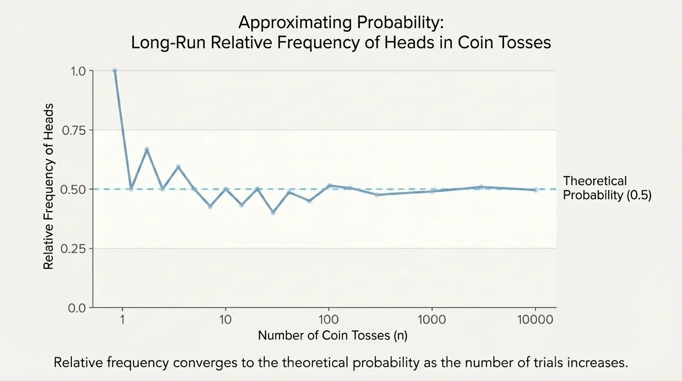
What becomes interesting is what happens when the number of trials grows. As [Figure 1] suggests, a coin flipped only a few times may look very unbalanced, but a coin flipped hundreds or thousands of times usually gives a much more even pattern. Probability does not remove variation, but it helps us understand the overall trend.
Probability describes how likely an event is to happen. For a fair chance process, the probability of an event is the number of favorable outcomes divided by the total number of possible outcomes. When we repeat a chance process many times, the observed results may bounce around at first but usually settle near the probability value.
For example, the probability of rolling an even number on a fair number cube is \(\dfrac{3}{6} = \dfrac{1}{2}\), because the favorable outcomes are \(2, 4, 6\). The probability of drawing a red marble from a bag with \(3\) red marbles and \(7\) blue marbles is \(\dfrac{3}{10}\).
Theoretical probability is the probability found by reasoning about all possible outcomes in a fair chance process.
Relative frequency is the fraction or ratio of times an event actually occurs in repeated trials.
The formula for relative frequency is
\[\textrm{relative frequency} = \frac{\textrm{number of times the event occurs}}{\textrm{total number of trials}}\]
If a coin is flipped \(50\) times and heads appears \(28\) times, the relative frequency of heads is \(\dfrac{28}{50} = 0.56\). This is not exactly \(0.5\), but it is fairly close. Experimental data often differ from theoretical probability because real results include random variation.
The idea of long-run relative frequency means that as the number of trials becomes large, the relative frequency tends to get closer to the theoretical probability. It may not move smoothly, and it may never become exact, but it usually gets closer overall.
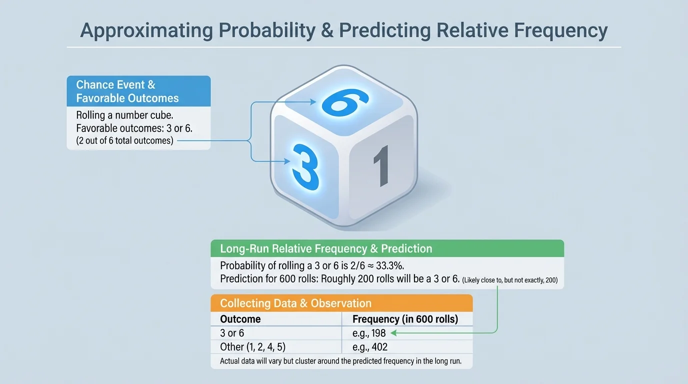
[Figure 2] One of the most useful probability skills is turning a probability into an approximate count. If you know the probability of an event and the number of trials, you can predict how many times the event should happen. When the event is rolling a \(3\) or \(6\) on a fair number cube, there are \(2\) favorable outcomes out of \(6\) total outcomes.
The basic prediction rule is
\[\textrm{predicted number of successes} = \textrm{probability} \times \textrm{number of trials}\]
If the probability of success is \(\dfrac{1}{4}\) and you run \(80\) trials, then the predicted number of successes is \(\dfrac{1}{4} \times 80 = 20\). This does not mean the event must happen exactly \(20\) times. It means \(20\) is a reasonable estimate.
Worked example 1
A fair number cube is rolled \(600\) times. Predict how many times a \(3\) or \(6\) will be rolled.
Step 1: Find the probability of the event.
The favorable outcomes are \(3\) and \(6\), so there are \(2\) favorable outcomes out of \(6\) total outcomes.
\[P(3 \textrm{ or } 6) = \frac{2}{6} = \frac{1}{3}\]
Step 2: Multiply by the number of trials.
Use the prediction rule: \(\dfrac{1}{3} \times 600 = 200\).
Step 3: Interpret the result.
The event should happen about \(200\) times.
The prediction is approximately \(200\) times, not exactly \(200\) times.
This example is important because it shows the difference between a mathematical expectation and actual data. If the result were \(196\), \(203\), or \(211\), those would still be reasonable outcomes.
Worked example 2
A fair coin is flipped \(150\) times. Predict how many times it lands on heads.
Step 1: Find the probability of heads.
For a fair coin, \(P(\textrm{heads}) = \dfrac{1}{2}\).
Step 2: Multiply by the number of trials.
\(\dfrac{1}{2} \times 150 = 75\).
Step 3: State the prediction clearly.
Heads should occur about \(75\) times.
The predicted relative frequency is \(0.5\), and the predicted count is about \(75\).
Notice that the count is found by multiplying probability by total trials. This same method works for dice, spinners, card draws, or any repeated chance process.
Worked example 3
A spinner has \(4\) equal sections: red, blue, green, and yellow. It is spun \(120\) times. Predict how many times it will land on blue or green.
Step 1: Identify favorable outcomes.
Blue and green are \(2\) favorable sections out of \(4\) equal sections.
\[P(\textrm{blue or green}) = \frac{2}{4} = \frac{1}{2}\]
Step 2: Multiply by the number of spins.
\(\dfrac{1}{2} \times 120 = 60\).
Step 3: Write the prediction.
The spinner should land on blue or green about \(60\) times.
A result such as \(57\) or \(63\) would still be close to the prediction.
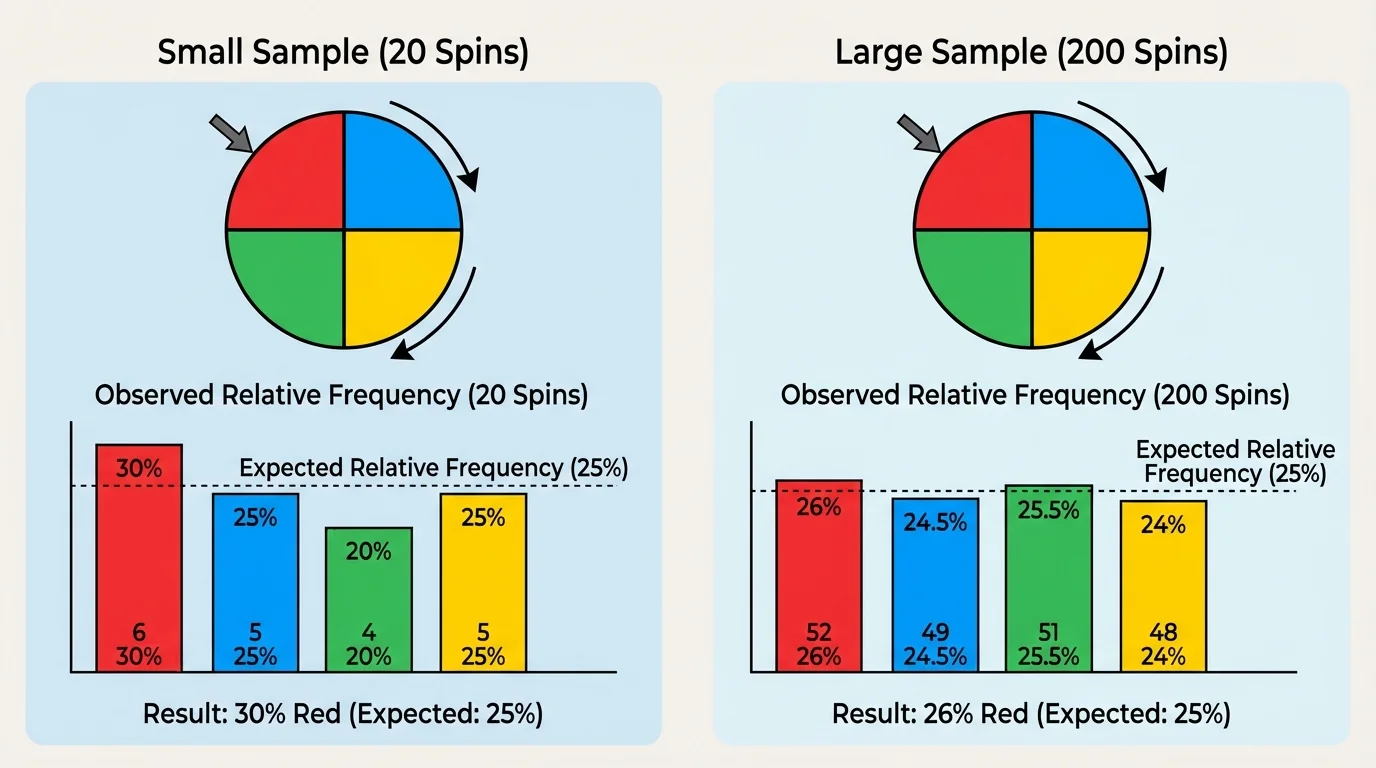
[Figure 3] Here is the big idea of this topic: repeated data can be used to approximate probability, and known probability can be used to predict repeated data. As the number of trials increases, the relative frequency often becomes more stable and usually moves closer to the theoretical probability.
Suppose a spinner has a \(\dfrac{1}{4}\) chance of landing on red. In \(20\) spins, red might appear \(8\) times, giving a relative frequency of \(\dfrac{8}{20} = 0.4\). That seems far from \(0.25\). But in \(200\) spins, red might appear \(52\) times, giving \(\dfrac{52}{200} = 0.26\), which is much closer.
This does not mean larger samples are always perfect. A result can still be a little high or low. The important idea is that larger samples usually give better estimates of the actual probability than smaller samples do.
Why "about" matters
Probability gives an expected pattern, not an exact promise. If an event has probability \(0.3\), then in \(100\) trials we predict about \(30\) successes because \(0.3 \times 100 = 30\). But random variation means the actual result might be \(27\), \(31\), or \(35\). "About" is a key word in probability.
This is why people collect lots of data before making decisions. A small set of results can be misleading, while a larger set is usually more trustworthy. Scientists, engineers, and statisticians depend on this idea when they study experiments and real-world events.
When you collect data from a chance process, you can compare the observed relative frequency with the theoretical probability. This helps you decide whether the experiment seems fair and whether the results are reasonable.
| Chance process | Event probability | Number of trials | Predicted count | Observed count | Observed relative frequency |
|---|---|---|---|---|---|
| Fair coin | \(\dfrac{1}{2}\) | \(40\) | \(20\) | \(18\) | \(\dfrac{18}{40} = 0.45\) |
| Fair number cube | \(\dfrac{1}{3}\) | \(60\) | \(20\) | \(23\) | \(\dfrac{23}{60} \approx 0.383\) |
| Four-section spinner | \(\dfrac{1}{4}\) | \(100\) | \(25\) | \(24\) | \(\dfrac{24}{100} = 0.24\) |
Table 1. Predicted and observed results for several chance processes.
In the table, none of the observed counts match the predicted counts exactly. That is normal. The key question is whether they are reasonably close. The spinner result of \(24\) out of \(100\) is very close to the prediction of \(25\). The number cube result of \(23\) out of \(60\) is a little farther away, but still possible.
Looking back at [Figure 1], we see the same pattern: data can wobble above and below the expected value before settling near it over time. Interpreting probability means understanding both the prediction and the natural variation around it.
Probability and relative frequency are not just classroom ideas. Meteorologists compare predicted chances of rain with actual weather data. A forecast of \(30\%\) rain does not mean it must rain on exactly \(30\%\) of a single day; it means that across many similar situations, rain happens about \(30\%\) of the time.
Sports analysts use shooting percentages in a similar way. If a player has a free-throw probability of \(0.8\), then in \(50\) shots we predict about \(0.8 \times 50 = 40\) made shots. The player may make \(38\) or \(43\), but \(40\) is the approximate expectation.
In medicine, researchers test how often a treatment works in many patients. In manufacturing, companies track the relative frequency of defective items to judge quality control. In gaming and technology, programmers use probability to balance random events so that the game feels fair over many plays.
Casinos make money because they understand long-run probability extremely well. A player might win in the short run, but over many games the results tend to follow the probabilities built into the games.
The same reasoning also helps people detect problems. If a coin that should land heads with probability \(\dfrac{1}{2}\) keeps giving heads about \(90\%\) of the time over hundreds of flips, that result is so far from the expected pattern that the coin may not be fair.
One misunderstanding is thinking that probability tells the exact result. It does not. If the probability of an event is \(\dfrac{1}{3}\) and you do \(300\) trials, the prediction is about \(100\) successes, but the actual number may differ.
Another misunderstanding is believing that short-run results must look balanced. A fair coin can land on heads \(5\) times in a row. That does not automatically mean the coin is unfair. Short runs can be surprising.
A third misunderstanding is assuming that a past result forces the next one. If a fair coin lands tails \(4\) times in a row, the probability of heads on the next flip is still \(\dfrac{1}{2}\). The coin has no memory.
Worked example 4
A bag contains \(5\) red marbles and \(15\) blue marbles. One marble is drawn, the color is recorded, and the marble is returned. This is repeated \(200\) times. Predict how many times a red marble will be drawn.
Step 1: Find the probability of drawing red.
There are \(5\) red marbles out of \(20\) total marbles.
\[P(\textrm{red}) = \frac{5}{20} = \frac{1}{4}\]
Step 2: Multiply by the number of trials.
\(\dfrac{1}{4} \times 200 = 50\).
Step 3: Interpret the result.
Red should be drawn about \(50\) times.
If the experiment gives \(47\) reds, that is still close to the prediction.
Because the marble is returned each time, the draws are made with replacement. That keeps the probability the same from one trial to the next. When conditions stay the same, repeated trials are easier to compare.
Probability can go in two directions. First, if you know the structure of a fair chance process, you can calculate a probability and predict an approximate relative frequency or count. Second, if you collect data from many repeated trials, you can use the relative frequency to estimate the probability.
For example, if a mystery spinner lands on purple \(48\) times out of \(200\) spins, the relative frequency is \(\dfrac{48}{200} = 0.24\). That suggests the probability of landing on purple is about \(0.24\), especially if the \(200\) spins are part of a fair and consistent process. As we saw earlier with the larger samples in [Figure 3], bigger data sets usually make that estimate more reliable.
This relationship between probability and data is one of the most powerful ideas in statistics. It helps us make predictions, test fairness, understand experiments, and make decisions based on evidence instead of guesses.