If a class raffle has one winner and every student has exactly one ticket, is everyone equally likely to win? Yes—and that simple idea is the heart of a probability model. Probability helps us describe what should happen in a fair chance situation. It also helps us compare that prediction to what actually happens in real life, where results can be surprising in the short term.
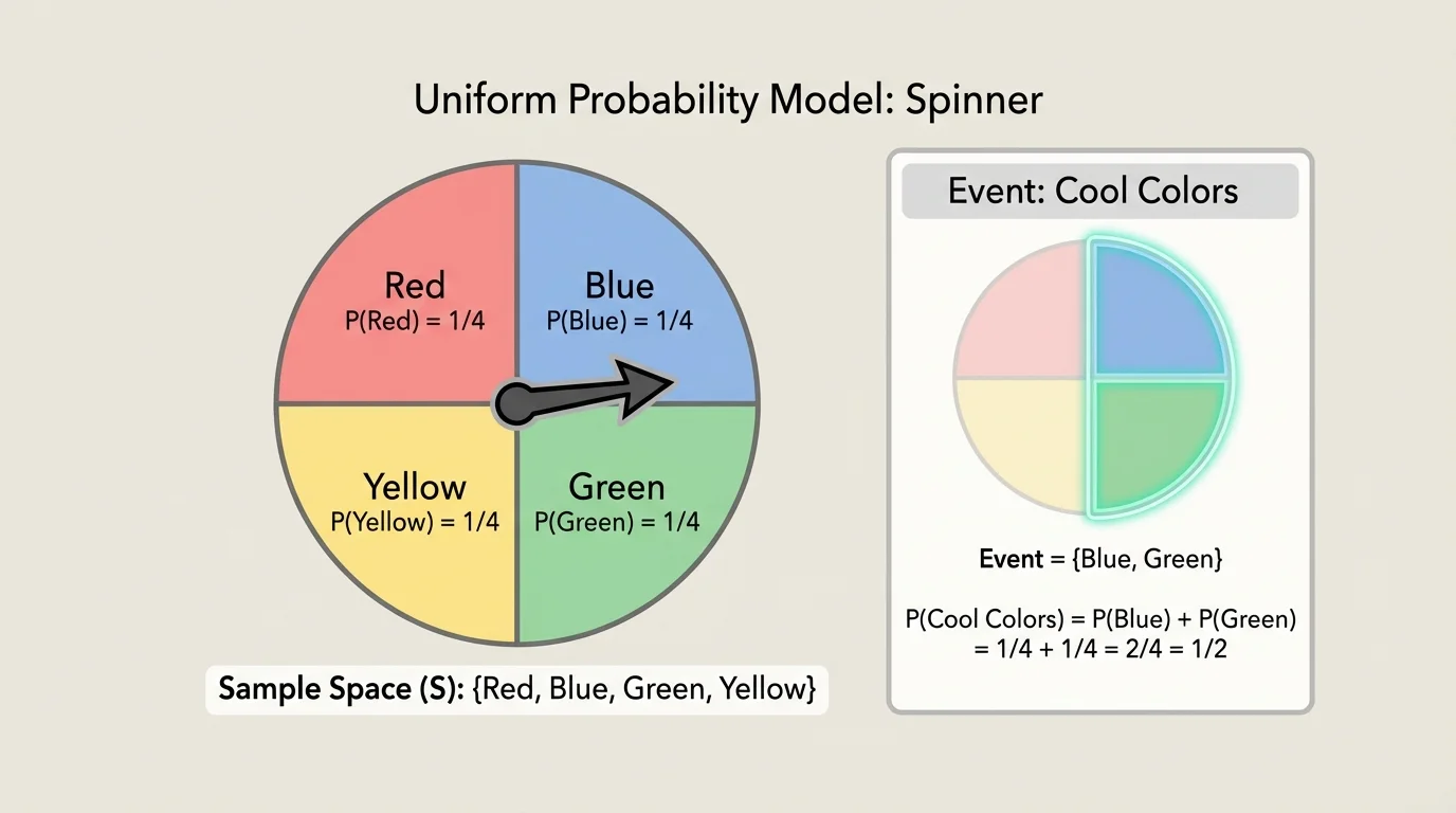
Probability begins with a chance process, such as rolling a number cube, spinning a spinner, or choosing a student at random. In any chance process, an outcome is one possible result. An event is a group of one or more outcomes that we care about. A sample space is the full list of all possible outcomes, as [Figure 1] shows with a simple spinner.
For example, suppose a spinner has four equal sections labeled red, blue, green, and yellow. The sample space is \(\{\textrm{red}, \textrm{blue}, \textrm{green}, \textrm{yellow}\}\). One outcome is landing on blue. An event could be "landing on a cool color," which includes blue and green. So that event has two outcomes.
When we study probability, it is important to know exactly what counts as one outcome. If a student is selected from a class, then each student is one outcome. If a number cube is rolled, then each number \(1, 2, 3, 4, 5, 6\) is one outcome. Clear outcomes lead to clear probability.
A uniform probability model is a probability model in which every outcome in the sample space has the same probability. If there are \(n\) equally likely outcomes, each outcome has probability \(\dfrac{1}{n}\).
Probability is a number from \(0\) to \(1\) that describes how likely an event is. A probability of \(0\) means impossible, and a probability of \(1\) means certain.
You already use probability language in everyday life. Saying something is "unlikely," "possible," or "almost certain" is informal probability. Mathematics turns those ideas into exact numbers.
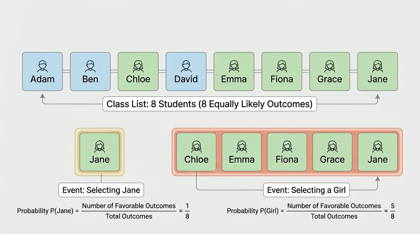
A uniform probability model works when every outcome is equally likely. This is true for a fair coin, a fair number cube, a spinner with equal sections, or a random selection where each person has the same chance. In the class-selection situation, [Figure 2] illustrates that each student represents one equally likely outcome.
When all outcomes are equally likely, we use a very useful rule:
\[P(\textrm{event}) = \frac{\textrm{number of favorable outcomes}}{\textrm{total number of outcomes}}\]
The favorable outcomes are the outcomes that make the event happen. The total number of outcomes is the size of the sample space.
Suppose there are \(8\) students in a class, and one student is selected at random. If every student has the same chance of being selected, then there are \(8\) equally likely outcomes. The probability that Jane is selected is \(\dfrac{1}{8}\), because Jane is one favorable outcome out of \(8\) possible outcomes.
Now suppose \(5\) of the \(8\) students are girls. The probability that a girl is selected is \(\dfrac{5}{8}\), because there are \(5\) favorable outcomes out of \(8\) total outcomes. Notice that "Jane is selected" is a single-outcome event, while "a girl is selected" is a multi-outcome event.
Uniform probability models are only valid when the outcomes really are equally likely. If one student has two raffle tickets while everyone else has one, then the outcomes are no longer equally likely. In that case, a uniform model would not fit the situation.
Fractions are a big part of probability. A fraction like \(\dfrac{3}{8}\) means \(3\) favorable outcomes out of \(8\) total outcomes. You can also write probabilities as decimals or percents, such as \(\dfrac{3}{8} = 0.375 = 37.5\%\).
Because probability measures chance, every probability must be between \(0\) and \(1\). A probability greater than \(1\) or less than \(0\) is impossible and means something went wrong in the setup or calculation.
When there is only one favorable outcome, the probability is often simple. For example, on a fair six-sided number cube, the probability of rolling a \(4\) is \(\dfrac{1}{6}\). But many events include more than one outcome. The probability of rolling an even number is \(\dfrac{3}{6}\), because the favorable outcomes are \(2, 4, 6\).
Probabilities can often be simplified. Since \(\dfrac{3}{6}\) and \(\dfrac{1}{2}\) represent the same amount, we can say the probability of rolling an even number is \(\dfrac{1}{2}\).
Another useful idea is the complement of an event. The complement is what does not happen. If the probability of selecting a girl is \(\dfrac{5}{8}\), then the probability of not selecting a girl is \(1 - \dfrac{5}{8} = \dfrac{3}{8}\). In a class with only girls and boys, that means the probability of selecting a boy is \(\dfrac{3}{8}\).
Complements are useful because sometimes it is easier to find the probability of the opposite event and subtract from \(1\). Since the total probability of all outcomes in the sample space is always \(1\), an event and its complement must add to \(1\).
Why the probabilities of all outcomes add to \(1\)
The sample space includes every possible result, so something in the sample space must happen. That means the total probability of all outcomes together is \(1\). In a uniform model with \(n\) equally likely outcomes, each has probability \(\dfrac{1}{n}\), and adding all \(n\) of them gives \(n \cdot \dfrac{1}{n} = 1\).
This idea also helps you check your work. If your listed probabilities for all outcomes do not add to \(1\), then the model or arithmetic needs to be fixed.
Examples are where probability becomes much more concrete. Notice how the same formula works in many different situations, including student selection, games, and surveys.
Worked example 1: Selecting a student from a class
A class has \(12\) students. One student is selected at random. Find the probability that Liam is selected and the probability that a girl is selected if \(7\) of the students are girls.
Step 1: Identify the total number of outcomes.
Each student is one equally likely outcome, so there are \(12\) total outcomes.
Step 2: Find the probability that Liam is selected.
Only one outcome is Liam, so \(P(\textrm{Liam}) = \dfrac{1}{12}\).
Step 3: Find the probability that a girl is selected.
There are \(7\) favorable outcomes, so \(P(\textrm{girl}) = \dfrac{7}{12}\).
The probabilities are \(\dfrac{1}{12}\) and \(\dfrac{7}{12}\).
Notice how this matches the class-selection model shown earlier in [Figure 2]. A single named student has one favorable outcome, but a group such as all girls may include several favorable outcomes.
Worked example 2: A fair spinner
A fair spinner has \(8\) equal sections labeled \(1\) through \(8\). Find the probability of landing on a number greater than \(5\).
Step 1: List the outcomes in the event.
Numbers greater than \(5\) are \(6, 7, 8\). There are \(3\) favorable outcomes.
Step 2: Count the total outcomes.
There are \(8\) equal sections, so there are \(8\) total outcomes.
Step 3: Write the probability.
\[P(\textrm{number greater than }5) = \frac{3}{8}\]
The probability is \(\dfrac{3}{8}\).
The spinner in [Figure 1] uses colors instead of numbers, but the reasoning is exactly the same: count the favorable sections and divide by the total number of equal sections.
Worked example 3: Choosing a card
A bag contains \(10\) cards numbered \(1\) through \(10\). One card is chosen at random. Find the probability of choosing an even number.
Step 1: Identify the favorable outcomes.
The even numbers are \(2, 4, 6, 8, 10\), so there are \(5\) favorable outcomes.
Step 2: Identify the total outcomes.
There are \(10\) cards in all.
Step 3: Form the probability and simplify.
The probability is \(\dfrac{5}{10}\), which simplifies to \(\dfrac{1}{2}\).
The probability of choosing an even number is \(\dfrac{1}{2}\).
Simplifying probabilities can make them easier to compare. For instance, \(\dfrac{5}{10}\) and \(\dfrac{1}{2}\) mean the same chance, but \(\dfrac{1}{2}\) is usually easier to recognize.
Worked example 4: Using a complement
A fair number cube is rolled once. Find the probability of not rolling a \(6\).
Step 1: Find the probability of rolling a \(6\).
There is \(1\) favorable outcome out of \(6\), so \(P(6) = \dfrac{1}{6}\).
Step 2: Use the complement.
The probability of not rolling a \(6\) is \(1 - \dfrac{1}{6} = \dfrac{5}{6}\).
The probability is \(\dfrac{5}{6}\).
Complements save time, especially when an event includes many outcomes. It is often faster to subtract a small probability from \(1\) than to count many favorable outcomes one by one.
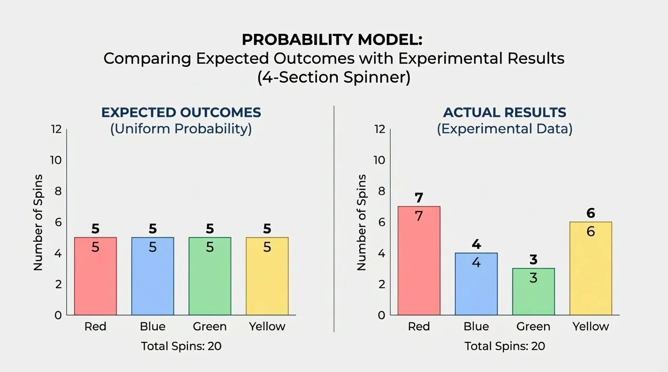
[Figure 3] Probability models tell us what we expect in the long run, but actual experiments may not match perfectly every time. This difference between a model and real data matters in statistics. The model gives a prediction, and the data show the observed frequency.
Suppose a fair spinner has \(4\) equal sections. The model says each color has probability \(\dfrac{1}{4}\). If you spin it \(20\) times, you might not get each color exactly \(5\) times. One possible result is red \(7\) times, blue \(4\) times, green \(3\) times, and yellow \(6\) times. Those are the observed frequencies.
Even if the spinner is fair, short runs can be uneven. Chance naturally creates variation. If you keep spinning many more times, the observed frequencies usually get closer to the model probabilities. This is why probability is often described as a long-run idea.
We can compare observed frequency to probability using fractions. In the example above, red appeared \(7\) out of \(20\) times, so the observed frequency for red is \(\dfrac{7}{20}\). The model predicted \(\dfrac{1}{4} = \dfrac{5}{20}\). These are not equal, but they are reasonably close for only \(20\) spins.
Why a model and data may disagree
If a probability model and the observed results do not agree well, there are several possible reasons: the number of trials may be small, the chance process may not be truly fair, or errors may have happened during the experiment or recording of data.
For example, if a coin is expected to land heads with probability \(\dfrac{1}{2}\), but in \(10\) flips it lands heads \(8\) times, that does not automatically mean the coin is unfair. But if in \(1{,}000\) flips it lands heads \(820\) times, then the disagreement is much more suspicious.
| Situation | Model probability | Observed frequency example | Possible explanation |
|---|---|---|---|
| Fair coin, \(10\) flips | Heads: \(\dfrac{1}{2}\) | \(\dfrac{8}{10}\) | Small sample, normal variation |
| Fair spinner, \(20\) spins | Each color: \(\dfrac{1}{4}\) | One color: \(\dfrac{7}{20}\) | Short-run randomness |
| Supposedly fair coin, \(1{,}000\) flips | Heads: \(\dfrac{1}{2}\) | \(\dfrac{820}{1{,}000}\) | Coin may be biased or data may be flawed |
Table 1. Examples comparing theoretical model probabilities with observed frequencies and possible reasons for disagreement.
The bar chart in [Figure 3] makes this idea easier to see: expected results and actual results may differ, but that difference does not always mean the model is wrong.
Uniform probability models appear in many real situations. Schools use random selection for class jobs, tournament pairings, or raffle prizes. Scientists use random sampling when they want to make fair choices in experiments. Game designers rely on probability to test whether a board game or digital game feels balanced and fair.
Surveys also use random selection. If every student in a school has an equal chance of being chosen for a survey, then a uniform model describes the selection process. The probability that one specific student is chosen is small, but every student has the same chance.
Professional sports analysts use probability models all the time. They estimate the chance of a team winning, a player making a shot, or a strategy paying off, even though the exact result of a single play can still be unpredictable.
Probability is also useful in quality testing. If one item is selected at random from a batch and each item is equally likely to be chosen, the selection follows a uniform model. Engineers and manufacturers use this kind of random selection to check product quality fairly.
One common mistake is assuming outcomes are equally likely when they are not. For example, if a spinner has one large section and three small sections, you should not assign each section probability \(\dfrac{1}{4}\). Equal-looking labels do not matter; equal-sized sections do.
Another mistake is mixing up an outcome with an event. "Jane is selected" is one outcome. "A girl is selected" may include several outcomes. The event's probability depends on how many favorable outcomes it contains.
A third mistake is using the wrong total number of outcomes. If there are \(15\) students in a class, you must divide by \(15\), not by the number of girls or boys alone unless that is the full sample space.
Careful probability work always asks three questions: What are all the possible outcomes? Are they equally likely? Which outcomes are favorable for the event? If you can answer those three questions clearly, you can usually build the right model and find the correct probability.
"Probability is not about predicting one exact result. It is about describing how likely results are in a fair chance process."
That is why probability can feel surprising. A fair process does not guarantee a perfectly balanced short-term pattern. It guarantees that the model gives the correct chances over many trials.