A medical test can sound impressive if you hear, "The result was positive." But the next question goes deeper: "Positive given what information?" The answer to "what do we already know happened?" changes everything. That shift is the heart of conditional probability. Instead of looking at all possible outcomes, we narrow our view to the outcomes that fit a certain condition, and then ask how many of those also satisfy another event.
Conditional probability matters because real decisions almost never happen in a vacuum. A coach asks for the probability that a player scores given that they took the penalty kick. A doctor asks for the probability a patient has a disease given a test result. A meteorologist asks for the probability of rain given a certain pressure system. In each case, the condition changes the universe of outcomes we are considering.
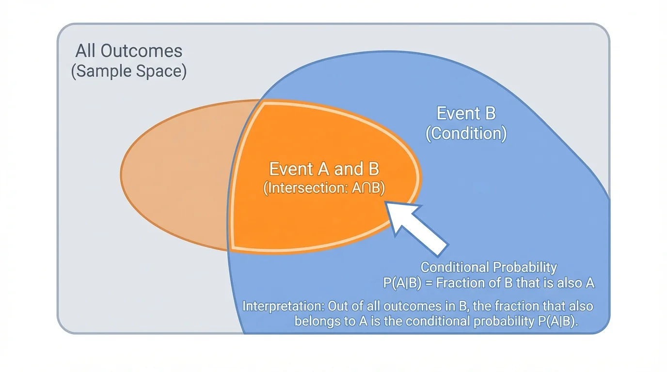
In an ordinary probability question, we begin with a sample space, the full set of possible outcomes. But in a conditional probability question, we are told that some event has already happened. Once that event occurs, as [Figure 1] shows, outcomes outside that event are no longer possible for the question we are asking. The condition acts like a filter.
Suppose event \(B\) has happened. Then we ignore every outcome not in \(B\). To find the probability of event \(A\) given \(B\), we count only the outcomes inside \(B\), and among those we see which also belong to \(A\). In other words, we ask: what fraction of the outcomes in \(B\) are also in \(A\)?
This idea is easier to understand if you think of a school directory. If you want the probability that a randomly chosen student plays soccer, you might divide the number of soccer players by the total number of students. But if you ask for the probability that a student plays soccer given that the student is in grade 11, then the total number of students is no longer the denominator. Now your denominator is only the number of grade 11 students.
That change in denominator is the key feature of conditional probability. The event after the word "given" determines the restricted set of outcomes.
Conditional probability is the probability that event \(A\) occurs given that event \(B\) has already occurred.
The notation is \(P(A\mid B)\), read as "the probability of \(A\) given \(B\)."
In a uniform probability model, where all outcomes are equally likely, \(P(A\mid B)\) is the fraction of outcomes in \(B\) that are also in \(A\).
Notice the wording carefully. The phrase "given \(B\)" does not mean multiply by \(B\), and it does not mean list \(A\) and \(B\) together in any order. It means that \(B\) is assumed true, so all counting now happens inside \(B\).
In a uniform probability model, all outcomes are equally likely, so conditional probability can be found by counting outcomes. If there are \(n(B)\) outcomes in event \(B\), and \(n(A\cap B)\) outcomes that belong to both \(A\) and \(B\), then
\[P(A\mid B)=\frac{n(A\cap B)}{n(B)}\]
Here, \(A\cap B\) means the outcomes in both events. The symbol \(\cap\) stands for "intersection," which is the overlap between two events.
This formula only makes sense when \(P(B)>0\), or in counting terms, when \(n(B)\neq 0\). If event \(B\) never happens, there are no outcomes in \(B\), so you cannot talk about "the fraction of \(B\) outcomes" that also belong to \(A\).
Recall: In a uniform probability model, probability is often found by counting equally likely outcomes: \(P(E)=\dfrac{\textrm{number of favorable outcomes}}{\textrm{total number of outcomes}}\). Conditional probability uses the same idea, but the "total number of outcomes" changes to the number of outcomes in the condition.
You can think of conditional probability as a two-step question. First, narrow the sample space to event \(B\). Second, inside that smaller world, count the outcomes that also satisfy \(A\).
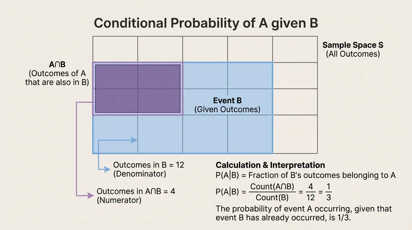
Sometimes the counting idea becomes much clearer when outcomes are displayed visually. In [Figure 2], equally likely outcomes are arranged in a grid, with event \(B\) highlighted and the overlap \(A\cap B\) marked separately. This makes conditional probability feel less mysterious: you are literally counting the overlap inside the conditioned set.
For example, suppose a model has \(20\) equally likely outcomes. If \(8\) outcomes are in \(B\), and \(3\) of those are also in \(A\), then the conditional probability is not \(\dfrac{3}{20}\). That would use the wrong denominator. The correct probability is \(\dfrac{3}{8}\), because only the outcomes in \(B\) are still under consideration.
This is one reason why conditional probability can feel counterintuitive at first. The same overlap \(A\cap B\) may lead to different answers depending on which event is being used as the condition. The numerator often stays the same, but the denominator changes.
When you interpret your answer, always include the condition in words. A value like \(\dfrac{3}{8}\) does not just mean "three out of eight." It means "among the outcomes where \(B\) happens, three out of eight also have \(A\)."
Let a fair six-sided die be rolled once. Define event \(A\): rolling an even number, and event \(B\): rolling a number greater than \(3\). Find \(P(A\mid B)\).
Worked example
Step 1: List the outcomes in \(B\).
The numbers greater than \(3\) are \(\{4,5,6\}\). So \(n(B)=3\).
Step 2: Find the outcomes that are in both \(A\) and \(B\).
Event \(A\) is the even numbers \(\{2,4,6\}\). The overlap with \(B\) is \(\{4,6\}\). So \(n(A\cap B)=2\).
Step 3: Form the conditional probability.
\[P(A\mid B)=\frac{n(A\cap B)}{n(B)}=\frac{2}{3}\]
The probability is \(\dfrac{2}{3}\).
The interpretation matters just as much as the calculation: among rolls greater than \(3\), two out of the three possible outcomes are even. So if you already know the roll is greater than \(3\), an even result is fairly likely.
If you compare this with the ordinary probability \(P(A)=\dfrac{3}{6}=\dfrac{1}{2}\), you can see how the condition changes the answer. Knowing the roll is greater than \(3\) increases the chance of an even number from \(\dfrac{1}{2}\) to \(\dfrac{2}{3}\).
A standard deck has \(52\) cards. Let event \(A\): drawing a queen, and event \(B\): drawing a face card. Find \(P(A\mid B)\).
Worked example
Step 1: Count the outcomes in \(B\).
Face cards are jacks, queens, and kings. There are \(3\) face cards in each of \(4\) suits, so \(n(B)=12\).
Step 2: Count the outcomes in \(A\cap B\).
Every queen is a face card, and there are \(4\) queens, so \(n(A\cap B)=4\).
Step 3: Compute the probability.
\[P(A\mid B)=\frac{4}{12}=\frac{1}{3}\]
The probability is \(\dfrac{1}{3}\).
The interpretation is: if you already know the card is a face card, then one-third of those face cards are queens. Notice how different this is from the ordinary probability of drawing a queen from the whole deck, which is \(\dfrac{4}{52}=\dfrac{1}{13}\).
Conditional probability is one of the ideas behind machine learning systems and medical decision-making. Many predictions are really answers to questions of the form "What is the probability of this outcome given the information we already have?"
This example also highlights a useful observation. If \(A\) is entirely contained in \(B\), then \(A\cap B=A\). In that case, the conditional probability becomes \(P(A\mid B)=\dfrac{P(A)}{P(B)}\), as long as \(P(B)>0\).
Suppose a school surveys \(100\) students. Let event \(A\): the student is in band, and event \(B\): the student plays a sport. The data are shown below.
| Group | In band | Not in band | Total |
|---|---|---|---|
| Plays a sport | 18 | 42 | 60 |
| Does not play a sport | 12 | 28 | 40 |
| Total | 30 | 70 | 100 |
Table 1. Student counts by band membership and sports participation.
Find \(P(A\mid B)\), the probability that a student is in band given that the student plays a sport.
Worked example
Step 1: Identify the conditioned group.
Because the question says "given that the student plays a sport," we only look at the \(60\) students who play a sport. So \(n(B)=60\).
Step 2: Find how many of those students are also in band.
Among the students who play a sport, \(18\) are in band. So \(n(A\cap B)=18\).
Step 3: Calculate the conditional probability.
\[P(A\mid B)=\frac{18}{60}=\frac{3}{10}=0.3\]
The probability is \(\dfrac{3}{10}\), or \(0.3\).
The correct interpretation is: among students who play a sport, \(30\%\) are in band. That is very different from saying "\(30\%\) of all students are in band," even though the number \(30\) also appears in the table. The condition determines which total you must use.
This kind of question appears often in data analysis, especially in two-way tables. The row total or column total used in the denominator depends on the phrase after "given."
[Figure 3] A common mistake is to think \(P(A\mid B)\) and \(P(B\mid A)\) are the same. They are not. The overlap \(A\cap B\) is the same region in both cases, but the reference set changes. In \(P(A\mid B)\), the denominator comes from \(B\). In \(P(B\mid A)\), the denominator comes from \(A\).
Using the club table above, \(P(\textrm{band}\mid \textrm{sport})=\dfrac{18}{60}=\dfrac{3}{10}\). But \(P(\textrm{sport}\mid \textrm{band})=\dfrac{18}{30}=\dfrac{3}{5}\). Same overlap, different denominator, different answer.
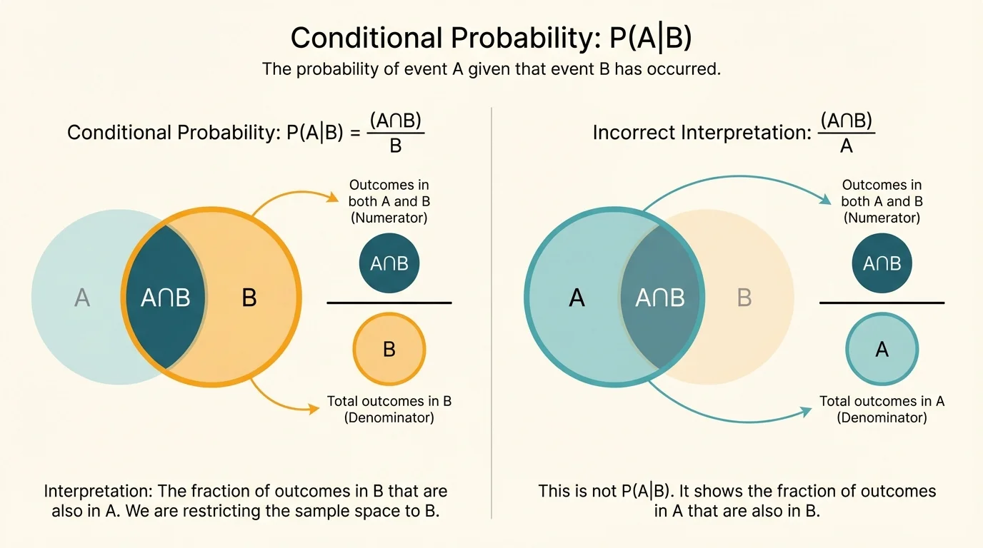
This difference matters a lot in real life. The probability of having a disease given a positive test is not the same as the probability of testing positive given the disease. Those two questions sound similar, but they are mathematically different.
Later, when you revisit more advanced probability, this distinction becomes central in topics like Bayes' theorem. For now, the most important habit is simple: read the order carefully.
In a uniform model, we often find conditional probability by counting outcomes. But the same idea can be written using probabilities instead of counts. Since \(P(A\cap B)\) is the probability that both events happen, and \(P(B)\) is the probability of the conditioned event, we have
\[P(A\mid B)=\frac{P(A\cap B)}{P(B)}\]
again assuming that \(P(B)>0\).
This formula matches the counting version. If all outcomes are equally likely, then \(P(A\cap B)=\dfrac{n(A\cap B)}{n(S)}\) and \(P(B)=\dfrac{n(B)}{n(S)}\), where \(S\) is the sample space. Dividing gives
\[\frac{P(A\cap B)}{P(B)}=\frac{\frac{n(A\cap B)}{n(S)}}{\frac{n(B)}{n(S)}}=\frac{n(A\cap B)}{n(B)}\]
So the probability formula and the counting formula are really the same idea expressed in two different ways.
Why the denominator is \(P(B)\)
Conditional probability asks about event \(A\) inside the restricted world where \(B\) has already happened. Because \(B\) is now the whole reference set, the denominator must measure the size of \(B\), not the size of the original sample space.
This is the exact same shift we saw earlier: once the condition is known, the effective sample space becomes smaller.
Mistake 1: Using the total number of all outcomes in the denominator. In conditional probability, the denominator should come from the condition, not from the full sample space.
Mistake 2: Reversing the order of the events. The notation \(P(A\mid B)\) does not mean the same thing as \(P(B\mid A)\). The event after the vertical bar tells you the restricted set.
Mistake 3: Forgetting to interpret the answer in context. A correct numerical answer should be expressed in words. For example, "Among students who play a sport, \(30\%\) are in band."
Mistake 4: Trying to calculate \(P(A\mid B)\) when \(P(B)=0\). If the conditioned event cannot occur, conditional probability is not defined.
"The condition tells you what world you are living in."
— A useful principle for interpreting conditional probability
That sentence is worth remembering because it keeps the entire topic organized. Once you know what world you are in, the denominator usually becomes clear.
Conditional probability appears whenever new information changes what outcomes are possible. In sports analytics, a team might ask for the probability of winning given that it leads at halftime. In manufacturing, an engineer might ask for the probability that a product is defective given that it failed an inspection test. In weather forecasting, scientists estimate the probability of storms given certain atmospheric conditions.
It also appears in social science and economics. A researcher may compare the probability of college attendance given family income level, or the probability of employment given a certain training program. These are all conditional probabilities because the phrase "given" creates a restricted group.
Medical testing provides one of the most important applications. If a patient tests positive, the natural question is not just "How accurate is the test?" but "What is the probability the patient has the disease given this positive result?" That is a conditional probability. Even highly accurate tests can lead to surprising results when the condition changes the relevant population.
The visual comparison helps explain why these medical questions can be misunderstood: the overlap stays the same, but whether you divide by all people with the disease or all people with positive tests makes a major difference.
When you finish a conditional probability problem, always connect the number back to the model. If \(P(A\mid B)=\dfrac{2}{3}\), ask: two-thirds of which group? The answer is always the group represented by \(B\).
For example, in the die problem, \(\dfrac{2}{3}\) means that among rolls greater than \(3\), two-thirds are even. In the card problem, \(\dfrac{1}{3}\) means that among face cards, one-third are queens. In the club table, \(0.3\) means that among students who play a sport, \(30\%\) are in band.
Interpreting the answer this way keeps probability tied to meaning instead of treating it like a disconnected fraction. Probability is not only about calculation; it is about understanding what a number says about a situation.