A student guesses on every question of a five-question multiple-choice quiz. Most people would say, "You will probably do badly." But probability can say much more than that. It can predict how often the student gets exactly \(0\), \(1\), \(2\), \(3\), \(4\), or \(5\) answers correct, and it can even predict the student's average score over many repeated quizzes. That is the power of probability distributions and expected value: they turn uncertainty into something we can analyze, compare, and use to make decisions.
These ideas are especially useful when outcomes have different values attached to them. A test score, a game prize, an insurance payment, or a business decision all involve uncertain results. When we build a probability distribution, we describe all possible values of a random variable and the probability of each one. When we compute expected value, we find the long-run average result if the same situation were repeated many times.
In everyday life, people often focus on what is possible. Mathematics asks a sharper question: what is likely, and what is the average result over time? A probability distribution answers that question for a discrete situation by listing each possible value and its probability.
Suppose a game pays different prizes depending on the number rolled on a die. Or suppose a grading system gives points for correct answers and penalties for wrong ones. You should not judge the system by only one possible outcome. You should judge it by the full distribution and by the expected value.
Sample space is the set of all possible outcomes of a random process.
Random variable is a variable that assigns a numerical value to each outcome in the sample space.
Probability distribution is a list, table, or rule giving each possible value of a random variable and the probability of that value.
Expected value is the long-run average value of a random variable, found by multiplying each value by its probability and adding the results.
For this lesson, we focus on discrete random variables, which take countable values such as \(0\), \(1\), \(2\), and so on. The number of correct answers on a test is discrete because you can count it.
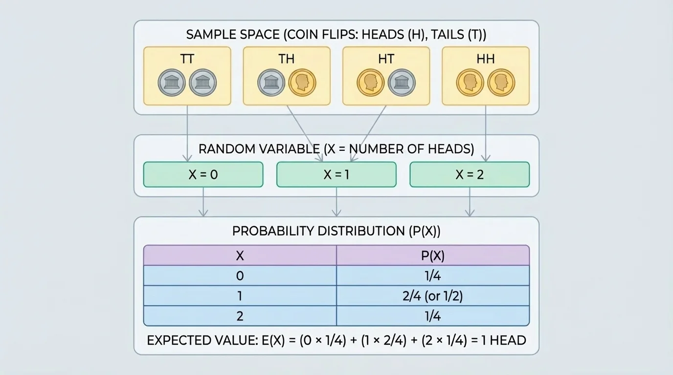
A sample space lists outcomes, but a random variable turns those outcomes into numbers. Several different outcomes can lead to the same value, as [Figure 1] illustrates. That is why we often start with the sample space and then group outcomes according to the value of the random variable.
For example, if two coins are tossed, the sample space is \(\{HH, HT, TH, TT\}\). Let \(X\) be the number of heads. Then \(X=0\) for outcome \(TT\), \(X=1\) for outcomes \(HT\) and \(TH\), and \(X=2\) for outcome \(HH\).
Because each of the four coin-toss outcomes is equally likely, we can find the probability distribution of \(X\):
| Value of \(X\) | Outcomes giving that value | Probability |
|---|---|---|
| \(0\) | \(TT\) | \(\dfrac{1}{4}\) |
| \(1\) | \(HT, TH\) | \(\dfrac{2}{4}=\dfrac{1}{2}\) |
| \(2\) | \(HH\) | \(\dfrac{1}{4}\) |
Table 1. Probability distribution for the number of heads in two coin tosses.
A valid probability distribution must satisfy two conditions: every probability is between \(0\) and \(1\), and the probabilities add to \(1\). Here, \(\dfrac{1}{4}+\dfrac{1}{2}+\dfrac{1}{4}=1\).
This simple example shows an important pattern: you do not assign probabilities directly to outcomes unless the random variable values are already clear. First identify the values the variable can take, then determine how likely each value is.
A probability distribution is called theoretical when the probabilities are calculated from mathematics rather than estimated from data. This happens when the sample space is known and outcomes are equally likely, or when the process follows a known probability model.
To build a theoretical probability distribution for a discrete random variable, follow this process:
Step 1: Identify the sample space or probability model.
Step 2: Define the random variable clearly.
Step 3: List all possible values of the random variable.
Step 4: Find the probability of each value.
Step 5: Check that all probabilities add to \(1\).
Sometimes each value comes from counting outcomes. In other cases, a formula gives the probability directly. In this lesson, the multiple-choice example uses a model called the binomial distribution, which applies when there is a fixed number of independent trials, each trial has two categories such as success or failure, and the probability of success stays constant.
How a binomial situation works
If there are \(n\) independent trials and the probability of success on each trial is \(p\), then the probability of getting exactly \(k\) successes is
\[P(X=k)=\binom{n}{k}p^k(1-p)^{n-k}\]
Here, \(\binom{n}{k}\) counts how many different ways the \(k\) successes can occur among the \(n\) trials.
For guessing on a multiple-choice question with four choices, a correct answer is a success with probability \(p=\dfrac{1}{4}\), and an incorrect answer is a failure with probability \(\dfrac{3}{4}\).
Now consider a five-question test where each question has four choices and only one correct answer. If a student guesses randomly on every question, the number of correct answers tends to cluster around lower values, as [Figure 2] shows later in this section. Let \(X\) be the number of correct answers.
Here, \(n=5\) and \(p=\dfrac{1}{4}\). So for each value \(k=0,1,2,3,4,5\),
\[P(X=k)=\binom{5}{k}\left(\frac{1}{4}\right)^k\left(\frac{3}{4}\right)^{5-k}\]
Solved example 1: Find the theoretical probability distribution for the number of correct answers
A student guesses on all five questions of a multiple-choice test with four choices per question.
Step 1: Identify the model
Each question is an independent trial. A correct guess has probability \(\dfrac{1}{4}\), so \(X\) follows a binomial model with \(n=5\) and \(p=\dfrac{1}{4}\).
Step 2: Compute each probability
For \(X=0\): \(P(X=0)=\binom{5}{0}\left(\dfrac{1}{4}\right)^0\left(\dfrac{3}{4}\right)^5=1\cdot 1\cdot \dfrac{243}{1024}=\dfrac{243}{1024}\).
For \(X=1\): \(P(X=1)=\binom{5}{1}\left(\dfrac{1}{4}\right)^1\left(\dfrac{3}{4}\right)^4=5\cdot \dfrac{1}{4}\cdot \dfrac{81}{256}=\dfrac{405}{1024}\).
For \(X=2\): \(P(X=2)=\binom{5}{2}\left(\dfrac{1}{4}\right)^2\left(\dfrac{3}{4}\right)^3=10\cdot \dfrac{1}{16}\cdot \dfrac{27}{64}=\dfrac{270}{1024}\).
For \(X=3\): \(P(X=3)=\binom{5}{3}\left(\dfrac{1}{4}\right)^3\left(\dfrac{3}{4}\right)^2=10\cdot \dfrac{1}{64}\cdot \dfrac{9}{16}=\dfrac{90}{1024}\).
For \(X=4\): \(P(X=4)=\binom{5}{4}\left(\dfrac{1}{4}\right)^4\left(\dfrac{3}{4}\right)^1=5\cdot \dfrac{1}{256}\cdot \dfrac{3}{4}=\dfrac{15}{1024}\).
For \(X=5\): \(P(X=5)=\binom{5}{5}\left(\dfrac{1}{4}\right)^5\left(\dfrac{3}{4}\right)^0=1\cdot \dfrac{1}{1024}\cdot 1=\dfrac{1}{1024}\).
Step 3: Check the total
\(\dfrac{243+405+270+90+15+1}{1024}=\dfrac{1024}{1024}=1\).
The probability distribution is valid.
We can organize the results in a table:
| Number correct \(x\) | Probability \(P(X=x)\) | Decimal approximation |
|---|---|---|
| \(0\) | \(\dfrac{243}{1024}\) | \(0.2373\) |
| \(1\) | \(\dfrac{405}{1024}\) | \(0.3955\) |
| \(2\) | \(\dfrac{270}{1024}\) | \(0.2637\) |
| \(3\) | \(\dfrac{90}{1024}\) | \(0.0879\) |
| \(4\) | \(\dfrac{15}{1024}\) | \(0.0146\) |
| \(5\) | \(\dfrac{1}{1024}\) | \(0.0010\) |
Table 2. Theoretical probability distribution for the number of correct answers when guessing on five four-choice questions.
This table reveals something interesting. The most likely result is not \(0\) correct but \(1\) correct. Also, getting all \(5\) correct by random guessing is extremely unlikely: only \(\dfrac{1}{1024}\).
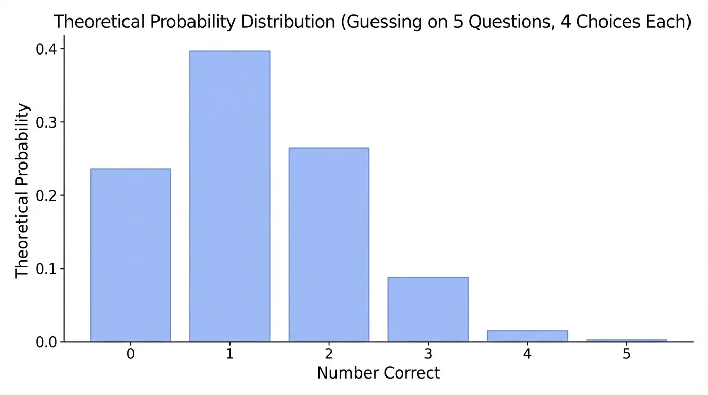
Notice that the distribution is not symmetric. Low scores are much more likely than high scores because the chance of a correct answer on each question is only \(\dfrac{1}{4}\). Later, when we discuss expected value, we will see that the long-run average is exactly what intuition suggests: a little more than one correct answer. In fact, in this case it is exactly \(\dfrac{5}{4}\), or \(1.25\).
The expected value of a discrete random variable \(X\) is found by multiplying each value by its probability and adding:
\[E(X)=\sum xP(X=x)\]
This does not mean the random variable must actually equal the expected value in one trial. For example, on a five-question test, a student cannot get exactly \(1.25\) questions correct. Expected value is a long-run average over many repetitions.
Solved example 2: Find the expected number of correct answers
Use the distribution from the five-question guessing situation.
Step 1: Write the expected value formula with the table values
\(E(X)=0\cdot \dfrac{243}{1024}+1\cdot \dfrac{405}{1024}+2\cdot \dfrac{270}{1024}+3\cdot \dfrac{90}{1024}+4\cdot \dfrac{15}{1024}+5\cdot \dfrac{1}{1024}\).
Step 2: Multiply and add
\(E(X)=\dfrac{0+405+540+270+60+5}{1024}=\dfrac{1280}{1024}=\dfrac{5}{4}\).
Step 3: Interpret the result
The expected number of correct answers is \(\dfrac{5}{4}=1.25\). Over many similar tests, a student who guesses on every question averages \(1.25\) correct answers per five-question test.
So the expected score is \(E(X)=1.25\).
There is also a shortcut for a binomial random variable. If \(X\) is binomial with \(n\) trials and success probability \(p\), then
\(E(X)=np\)
For the test, \(E(X)=5\cdot \dfrac{1}{4}=\dfrac{5}{4}=1.25\), which matches the value found from the full distribution.
Expected value is one of the main ideas behind casino games. A game can look attractive because of a possible large payout, but if the expected value is negative for the player, the casino has the advantage in the long run.
The same logic applies to grading. If a score depends on how many answers are correct or wrong, expected value tells us the average score a random guesser would receive.
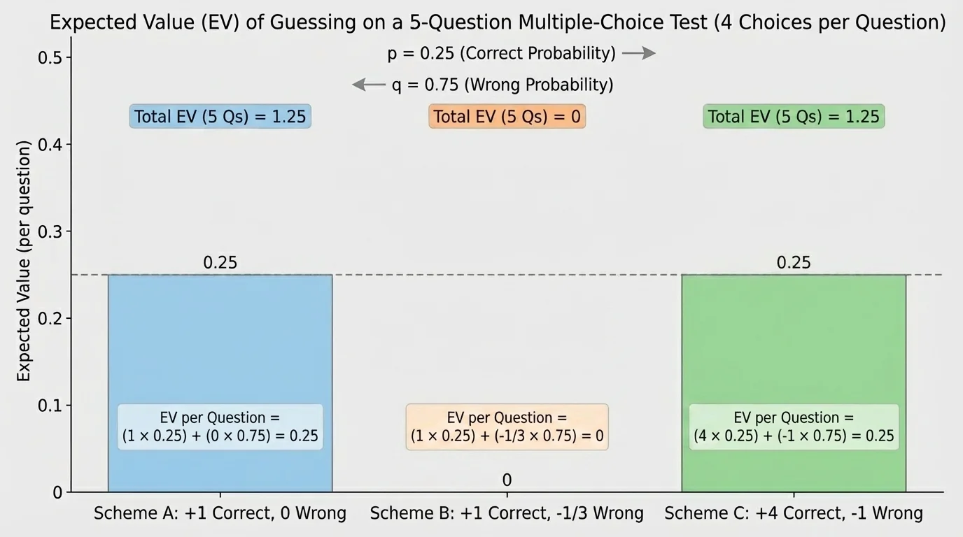
Different scoring rules can reward or punish guessing in very different ways, and [Figure 3] compares several common types. Expected value is the right tool because it combines both the points attached to outcomes and their probabilities.
Suppose a five-question test uses one of several grading schemes. We can define a new random variable for the score and then compute its expected value.
Solved example 3: Expected grade under three grading schemes
A student guesses on all five questions, with probability \(\dfrac{1}{4}\) of getting each question correct.
Step 1: Scheme A — \(1\) point for a correct answer, \(0\) points for a wrong answer
If \(X\) is the number correct, then score \(S=X\). So \(E(S)=E(X)=1.25\).
Step 2: Scheme B — \(1\) point for correct, \(-\dfrac{1}{3}\) point for wrong
For one question, the expected score is \(1\cdot \dfrac{1}{4}+\left(-\dfrac{1}{3}\right)\cdot \dfrac{3}{4}=\dfrac{1}{4}-\dfrac{1}{4}=0\).
For five questions, the expected score is \(5\cdot 0=0\).
Step 3: Scheme C — \(4\) points for correct, \(-1\) point for wrong
For one question, the expected score is \(4\cdot \dfrac{1}{4}+(-1)\cdot \dfrac{3}{4}=1-\dfrac{3}{4}=\dfrac{1}{4}\).
For five questions, the expected score is \(5\cdot \dfrac{1}{4}=\dfrac{5}{4}=1.25\).
Under these schemes, a random guesser averages \(1.25\), \(0\), and \(1.25\) points respectively.
Scheme B is especially important. A penalty of \(-\dfrac{1}{3}\) for a wrong answer exactly balances the advantage of random guessing when there are four choices. That means random guessing has expected value \(0\) per question. This kind of system is designed so that guessing does not help on average.
We can summarize these schemes in a compact table:
| Scheme | Scoring rule per question | Expected value per question | Expected value for \(5\) questions |
|---|---|---|---|
| A | Correct: \(1\), Wrong: \(0\) | \(\dfrac{1}{4}\) | \(1.25\) |
| B | Correct: \(1\), Wrong: \(-\dfrac{1}{3}\) | \(0\) | \(0\) |
| C | Correct: \(4\), Wrong: \(-1\) | \(\dfrac{1}{4}\) | \(1.25\) |
Table 3. Comparison of expected values for different grading schemes when each question has four answer choices.
This shows how expected value supports decision-making. If a teacher wants to discourage blind guessing, a penalty can be chosen so that the expected gain from guessing is zero. If a game designer wants a game to favor the house, the expected value can be set negative for the player.
To see that this topic is broader than tests, consider a simple game. You roll a fair six-sided die and define \(Y\) as the amount won in dollars: \(\$0\) for rolling \(1,2,3\), \(\$5\) for rolling \(4,5\), and \(\$20\) for rolling \(6\). The random variable values are \(0\), \(5\), and \(20\).
Solved example 4: Expected value of a game payout
Find the expected payout.
Step 1: Write the distribution
\(P(Y=0)=\dfrac{3}{6}=\dfrac{1}{2}\), \(P(Y=5)=\dfrac{2}{6}=\dfrac{1}{3}\), and \(P(Y=20)=\dfrac{1}{6}\).
Step 2: Compute expected value
\(E(Y)=0\cdot \dfrac{1}{2}+5\cdot \dfrac{1}{3}+20\cdot \dfrac{1}{6}=0+\dfrac{5}{3}+\dfrac{10}{3}=\dfrac{15}{3}=5\).
Step 3: Interpret
The long-run average payout is $5 per play.
The expected payout is \(E(Y)=5\)
If the game costs more than $5 to play, it is a bad deal for the player in the long run. If it costs less than $5, it favors the player. This is the same decision-making logic used with grading systems and with the test-guessing problem.
Students often make a few predictable errors when working with distributions and expected value.
Mistake 1: Forgetting that probabilities must add to \(1\). A quick check can catch arithmetic errors.
Mistake 2: Confusing outcomes in the sample space with values of the random variable. In the coin example, \(HT\) and \(TH\) are different outcomes, but both give \(X=1\), as we saw earlier in [Figure 1].
Mistake 3: Thinking expected value must be a possible outcome. It does not. On the test, \(1.25\) correct answers is impossible in one trial, but it is the average over many trials.
Mistake 4: Mixing up theoretical and experimental probability. Theoretical probability comes from a known model. Experimental probability comes from observed data. If real students guess on actual tests, their results may differ from theory in small samples, but over many trials they should be close.
When outcomes are equally likely, probability can often be found by counting: \(P(\textrm{event})=\dfrac{\textrm{number of favorable outcomes}}{\textrm{total number of outcomes}}\). For repeated independent trials, multiplication and combinations are often needed.
Another useful check is to ask whether the expected value makes sense. On a five-question test with four choices each, an expected value much larger than \(5\) or negative would be impossible for the number correct. Reasonableness matters.
Probability distributions and expected value appear anywhere people must make choices under uncertainty.
Education: Test designers use expected value to think about scoring rules. The comparison in [Figure 3] shows how penalties can make random guessing neutral on average.
Insurance: Companies estimate expected payouts based on the probabilities of accidents, illness, or damage. Premiums must exceed expected payouts on average for the company to stay in business.
Business: A company launching a product may consider profits under different demand levels and then compute expected profit.
Games and gambling: Casinos rely on expected value to design games that earn money over time, even if players sometimes win large prizes.
Science and engineering: Reliability analysis uses probability distributions to estimate the expected number of failures in systems, from electronic devices to transportation networks.
All of these situations share the same structure: define a random variable, assign probabilities, calculate expected value, and use the result to make better decisions.