A lake can look full of life one year and nearly empty the next. A forest may support hundreds of deer for decades, then suddenly face starvation after a harsh winter. These changes are not random. They reflect a powerful ecological idea: every ecosystem has limits. Understanding those limits is one of the main ways scientists explain why populations rise, fall, or stay stable.
When a population has abundant food, water, space, and favorable conditions, it can grow quickly. But no real ecosystem provides unlimited resources. At some point, competition increases, waste builds up, disease spreads more easily, or weather conditions become stressful. Population growth slows because the environment cannot support unlimited individuals.
The maximum population size that an environment can support over time is called carrying capacity. In ecology, carrying capacity is often represented by the symbol carrying capacity, written as \(K\). If a meadow can support about \(200\) rabbits over many seasons, then its carrying capacity for rabbits is about \(K = 200\). That number is not a permanent rule; it depends on current conditions.
Carrying capacity matters because organisms interact constantly with both living and nonliving parts of the environment. Plants need light, water, mineral nutrients, and space. Herbivores need plants. Predators need prey. Decomposers recycle matter back into the system. If one part changes, the whole system can shift.
Carrying capacity is the largest population of a species that an ecosystem can support for an extended time using available resources.
Limiting factor is any biotic or abiotic factor that restricts population size, growth, or distribution.
Population size is the number of individuals of one species in a given area.
A useful way to think about carrying capacity is to compare an ecosystem to a battery in a device. If too many apps run at once, the battery drains faster than it can be recharged. In ecosystems, if a population uses resources faster than those resources are replaced, the system cannot keep supporting that population at the same level.
A population is a group of individuals of the same species living in the same area. Population size changes because of births, deaths, immigration, and emigration. A simple way to describe this is:
\(\textrm{population change} = \textrm{births} + \textrm{immigration} - \textrm{deaths} - \textrm{emigration}\).
Scientists often track these values with field observations, camera traps, mark-and-recapture data, nesting counts, or satellite images. The goal is not just to count organisms but to explain why the numbers change.
A limiting factor can be biotic, meaning it comes from living interactions, or abiotic, meaning it comes from nonliving conditions. Biotic factors include food availability, predation, competition, and disease. Abiotic factors include temperature, sunlight, water, soil nutrients, pH, salinity, fire, and storms.
Some limiting factors are density-dependent factors. Their effects become stronger as population density increases. Disease is a good example. If \(20\) deer live in a large forest, they may rarely encounter one another. If \(500\) deer crowd the same area, pathogens spread much more easily. Other factors are density-independent factors, such as hurricanes or droughts, which can affect populations regardless of how crowded they are.
From earlier ecology work, remember that organisms need matter and energy from the environment. Energy often enters ecosystems through photosynthesis, in which producers use sunlight to make sugars such as \(\textrm{C}_6\textrm{H}_{12}\textrm{O}_6\) from \(\textrm{CO}_2\) and \(\textrm{H}_2\textrm{O}\). Because energy transfer is limited at each trophic level, ecosystems cannot support unlimited biomass at higher levels.
Carrying capacity can be different for different species in the same place. A forest might support many insects, fewer birds, and even fewer large predators. That does not mean the forest is failing. It means energy and matter move through ecosystems in ways that create natural limits.
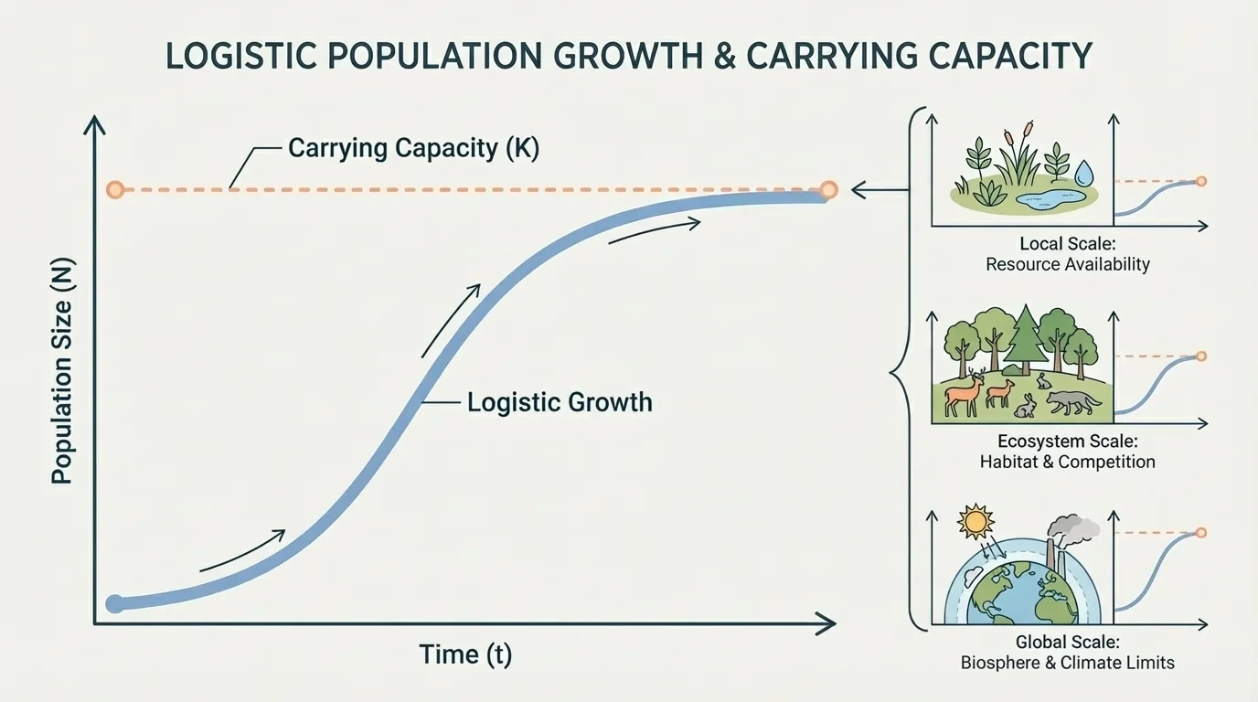
Ecologists often explain carrying capacity using graphs, tables, and simple calculations. A graph can reveal whether a population is growing rapidly, declining, or leveling off, as [Figure 1] shows for a population approaching an environmental limit. The goal is not to derive complex equations here, but to interpret what the representations mean.
One common pattern is fast growth at first, followed by slower growth as resources become limited. This pattern is called logistic growth. Early in growth, resources are abundant and the population rises quickly. Later, the growth rate decreases because competition and other limiting factors become stronger.
Suppose a yeast population in a lab culture changes like this over several days:
| Day | Population |
|---|---|
| \(1\) | \(100\) |
| \(2\) | \(180\) |
| \(3\) | \(300\) |
| \(4\) | \(420\) |
| \(5\) | \(470\) |
| \(6\) | \(490\) |
Table 1. Population data for yeast showing rapid increase followed by leveling near a limit.
The increase from day \(1\) to day \(2\) is \(180 - 100 = 80\). The increase from day \(5\) to day \(6\) is only \(490 - 470 = 20\). The slowing growth suggests the culture is nearing its carrying capacity, which appears to be close to \(500\).
Another useful representation is population density. If \(150\) prairie dogs live in an area of \(3\) square kilometers, the density is \(\dfrac{150}{3} = 50\) prairie dogs per square kilometer. Density helps explain why crowding can increase competition, disease transmission, and stress.
Scientists also compare proportions. If a fish population contains \(900\) juveniles and \(100\) adults, that age structure suggests future growth may be possible if enough juveniles survive. But if food is scarce, many may die before reproducing. Numbers alone do not explain the system; they must be interpreted with environmental conditions.
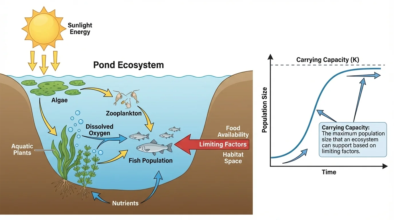
Carrying capacity becomes easier to understand when you examine actual ecosystems. A small pond, as shown in [Figure 2], can support only a certain number of fish because fish depend on dissolved oxygen, food organisms, water temperature, and space. If algae grow excessively and then decompose, oxygen levels can drop sharply, reducing the number of fish the pond can support.
Example 1: Fish in a pond
A pond contains \(40\) fish in spring and \(52\) fish in summer. By late summer, dissolved oxygen decreases, and the fish population falls to \(45\).
Step 1: Interpret the increase.
The increase from spring to summer is \(52 - 40 = 12\) fish, suggesting conditions were favorable at first.
Step 2: Interpret the decrease.
The decrease from summer to late summer is \(52 - 45 = 7\) fish. The likely limiting factor is reduced dissolved oxygen, an abiotic factor.
Step 3: Connect the data to carrying capacity.
If the pond repeatedly stabilizes around \(45\) to \(50\) fish, that range is a reasonable estimate of carrying capacity under those conditions.
This example shows that carrying capacity depends on both living and nonliving factors, not just on the amount of water in the pond.
At a larger scale, consider deer in a forest. Deer need vegetation, water, shelter, and enough area to move safely. If the forest provides enough plant growth to feed about \(800\) deer through a normal winter, then \(800\) is an approximate carrying capacity under those conditions. If a harsh winter kills many plants or covers food with ice, the carrying capacity may drop.
As the pond example and the forest example both show, carrying capacity is linked to resource supply. In a small system, one factor such as oxygen may matter most. In a larger system, several factors interact at once, including food, predators, parasites, and weather.
Example 2: Deer in a forest
A forest begins winter with \(900\) deer, but vegetation surveys suggest the habitat can support only about \(750\) deer through winter.
Step 1: Compare population to carrying capacity.
The population exceeds carrying capacity by \(900 - 750 = 150\) deer.
Step 2: Predict likely outcomes.
Competition for food will increase. Some deer may starve, become weaker and more vulnerable to disease, or migrate if possible.
Step 3: Explain the ecological meaning.
The problem is not that deer are "bad" for the ecosystem. The issue is that resource demand is greater than resource supply.
This is why wildlife managers monitor both population numbers and habitat quality.
At an even larger scale, ocean fisheries show that carrying capacity applies across huge ecosystems too. A region of ocean may support a certain biomass of sardines based on nutrient upwelling, plankton production, water temperature, and predator pressure. If harvest rates stay below the rate at which the population can recover, the fishery may remain stable. If harvest rates are too high, the population can fall below sustainable levels.
Carrying capacity is not controlled by a single factor. It emerges from many interacting conditions. Biotic factors include food supply, competitors, predators, parasites, disease-causing organisms, and availability of mates. Abiotic factors include temperature, rainfall, sunlight, nutrient availability, fire frequency, water chemistry, and natural disasters.
Suppose a grassland receives enough rainfall to produce \(1,200\) kilograms of plant biomass for grazers during one season. In a drought year, plant biomass might drop to \(700\) kilograms. If each antelope requires about \(10\) kilograms of usable plant biomass during that period, then the grassland might support about \(120\) antelope in the first case and only about \(70\) in the drought case. This is a simple estimate, but it shows how an abiotic factor can reduce carrying capacity.
Biotic interactions can shift carrying capacity too. If an invasive insect kills many trees in a forest, birds that nest in those trees may decline because habitat and food webs both change. If a predator disappears, herbivore numbers may rise temporarily, but then overgrazing may lower plant abundance and reduce carrying capacity later.
Why overshoot happens
Sometimes a population rises above carrying capacity for a short time. This is called an overshoot. It can happen after a season of unusual resource abundance or when predators are removed. Overshoot is often followed by a population crash because the ecosystem cannot keep supplying enough resources to maintain that high number.
These changes help explain why carrying capacity is better understood as a moving target than a fixed ceiling. Seasonal variation, climate shifts, nutrient cycling, and species interactions can all push the limit upward or downward.
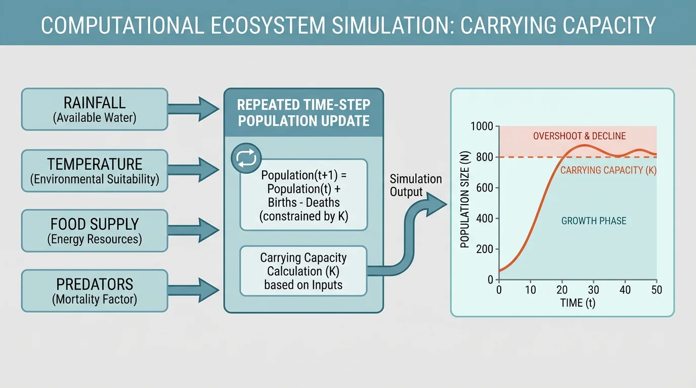
Many ecosystems are too complex to understand with one graph or one table alone. That is where computational models become useful. A simulation can update population size step by step based on conditions such as rainfall, food supply, predator numbers, and disease spread, as [Figure 3] illustrates. Scientists use these tools to test scenarios that would be difficult, expensive, or unethical to create in the real world.
A computational model is not a crystal ball. It is a representation built from assumptions, data, and rules. For example, a model may assume that if rainfall decreases, plant growth decreases; if plant growth decreases, herbivore survival decreases; and if herbivore survival decreases, predator numbers later decline as well.
Suppose a computer simulation predicts rabbit population size under three rainfall conditions:
| Rainfall condition | Predicted average rabbits supported |
|---|---|
| High | \(240\) |
| Moderate | \(180\) |
| Low | \(95\) |
Table 2. Model predictions showing how rainfall level changes the number of rabbits an ecosystem can support.
These outputs suggest that rainfall affects plant growth, which affects rabbit carrying capacity. The model does not prove the future exactly. It helps scientists explain likely outcomes and compare scenarios.
Example 3: Interpreting a drought simulation
A simulation starts with \(150\) rabbits. Under normal rainfall, the population stabilizes near \(180\). Under drought, it stabilizes near \(100\).
Step 1: Identify the modeled carrying capacities.
Normal conditions suggest \(K \approx 180\). Drought conditions suggest \(K \approx 100\).
Step 2: Compare the change.
The carrying capacity decreases by \(180 - 100 = 80\) rabbits.
Step 3: Explain the cause.
Drought is an abiotic factor that reduces plant growth and water availability, which lowers the ecosystem's ability to support rabbits.
This kind of model helps ecologists plan for future environmental stress.
Computational representations are especially important when multiple factors interact over time. A short drought may have little effect if soil moisture remains high, but a long drought combined with heat and disease may sharply reduce carrying capacity. Simulations help organize these interacting variables.
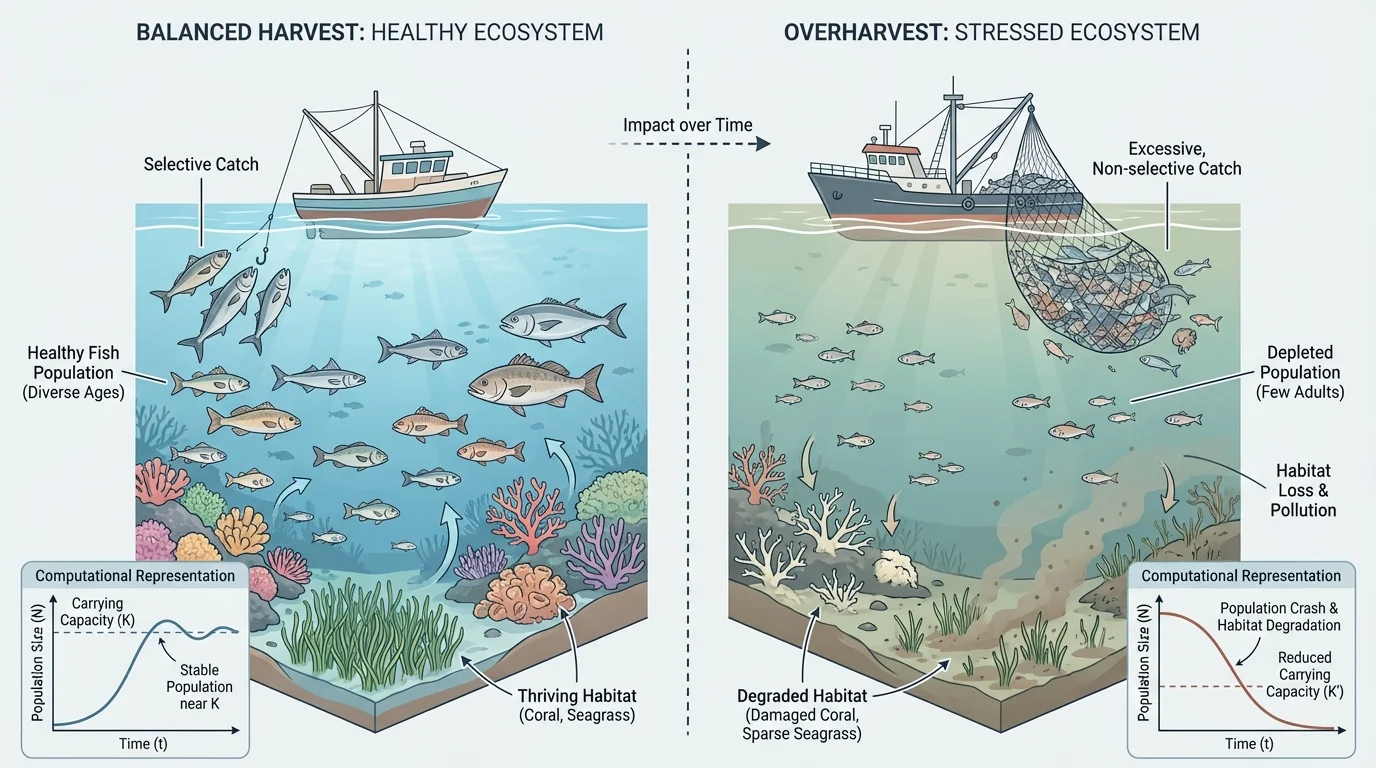
Carrying capacity is not just an abstract ecological idea. It guides real decisions about harvesting, habitat restoration, protected areas, and wildlife management. In fisheries, as [Figure 4] shows, managers try to avoid removing organisms faster than the population can recover under existing environmental conditions.
For example, if surveys estimate a fish population at \(1,000,000\) individuals and long-term data suggest the ecosystem can maintain about that number only when annual harvest stays moderate, managers may set catch limits. If ocean warming reduces plankton and juvenile survival, the carrying capacity may fall, and the same harvest level may become unsustainable.
Agriculture also involves carrying capacity. A pasture can support only a certain number of cattle before overgrazing reduces plant cover and soil quality. If a farmer places \(60\) cattle on land that can sustainably support only \(45\), the vegetation may not recover quickly enough. Soil erosion and lower productivity can follow, reducing future carrying capacity even more.
Urban ecosystems have carrying capacities too. A city park may support a certain number of squirrels, pigeons, or deer depending on food, nesting spaces, green area, and human disturbance. Feeding wildlife can temporarily increase local populations, but it may also increase disease transmission and conflict with humans.
Later, when conservation scientists revisit sustainable harvest or habitat restoration, the fisheries example in [Figure 4] remains useful because it shows that population numbers must be interpreted together with environmental support systems, not in isolation.
Some seabird colonies can shrink even when adult birds are still present in large numbers. The reason is that changes in ocean temperature may reduce fish availability, so fewer chicks survive. A stable-looking population can hide a declining carrying capacity.
It is tempting to treat carrying capacity as one exact number, but ecosystems rarely behave that neatly. A wetland may support more frogs in a rainy year than in a dry year. A forest recovering after fire may support fewer large mammals at first, then more as vegetation regrows. Migration can also change local population size without changing the total regional population.
At different scales, the same principle holds. A terrarium, a pond, a forest, a biome, or an ocean region all have limits based on matter, energy, and environmental conditions. The difference is that larger systems often involve more variables and more delayed effects. In a pond, oxygen changes may affect fish within hours. In a forest, nutrient depletion or predator decline may affect carrying capacity over years.
The graph of logistic growth in [Figure 1] is useful because it reminds us that slowing growth is often a sign that limiting factors are increasing. The pond system in [Figure 2] shows how those limiting factors can include both living interactions and nonliving conditions at the same time.
Mathematical and computational representations are valuable because they turn ecological ideas into evidence-based explanations. A table can show that growth slows. A calculation can show that resources per organism are falling. A graph can reveal a pattern across time. A computer model can test what happens if rainfall drops, predators increase, or disease spreads. Together, these tools help scientists explain why populations do not grow forever and why carrying capacity changes across ecosystems and across scales.
"Everything is connected to everything else."
— A core ecological principle
When scientists explain carrying capacity well, they are really answering a bigger question: how do organisms obtain enough matter and energy from the biotic and abiotic environment to survive together over time? The answer always depends on limits, interactions, and change.