Some functions rise smoothly forever. Others bounce, turn, or level off. But rational functions exhibit especially striking behavior: they can shoot upward near one value, plunge downward near another, and still settle into a predictable pattern far away. That combination of complex behavior near certain inputs and predictable behavior at the extremes makes them powerful tools in algebra, science, and engineering.
A rational function is any function that can be written as a quotient of two polynomials:
\[f(x)=\frac{P(x)}{Q(x)}\]
where \(P(x)\) and \(Q(x)\) are polynomials and \(Q(x)\neq 0\). The denominator cannot equal \(0\), so values that make \(Q(x)=0\) are not in the domain.
Factoring is the key skill for graphing many rational functions by hand. When the numerator and denominator are written in factored form, you can often read important graph features directly. For example, in \(f(x)=\dfrac{(x-3)(x+1)}{(x-2)(x+4)}\), the factors tell you where the function may equal \(0\) and where it is undefined.
To factor successfully, recall common techniques such as greatest common factor, difference of squares, and simple quadratic factoring. Also remember that an \(x\)-intercept happens when \(y=0\), while a vertical asymptote is connected to values that make the denominator \(0\).
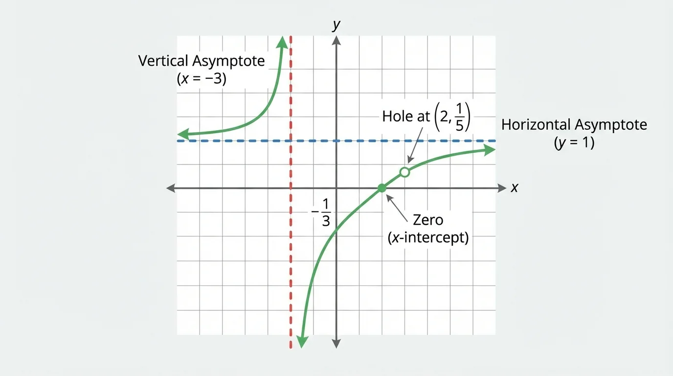
[Figure 1] Before graphing, it helps to separate what makes the output zero from what makes the output undefined. Those two ideas control much of the graph's shape.
The first things to look for are zeros, vertical asymptotes, and any hole in the graph. These features come directly from the factors, but you must handle common factors carefully.
Zeros occur when the numerator is \(0\) and the denominator is not \(0\). In factored form, set each numerator factor equal to \(0\). These usually become \(x\)-intercepts.
Vertical asymptotes usually occur at values of \(x\) that make the denominator \(0\), after simplifying any common factors. Near these values, the function often grows without bound, heading toward \(+\infty\) or \(-\infty\).
Holes occur when a factor cancels from the numerator and denominator. The original function is still undefined at that \(x\)-value, but instead of a vertical asymptote, the graph has a missing point on the simplified curve.
You should also find the y-intercept if it exists. Substitute \(x=0\) into the function, provided the denominator is not \(0\). This gives a useful anchor point for sketching.
An asymptote is a line that a graph approaches more and more closely. A vertical asymptote has equation \(x=a\), and a horizontal asymptote has equation \(y=b\). A slant asymptote is a diagonal line the graph approaches when the degree of the numerator is exactly one more than the degree of the denominator.
A canceled factor changes everything. If \(f(x)=\dfrac{(x-2)(x+1)}{(x-2)(x-3)}\), the factor \((x-2)\) cancels in the expression, but the original function is still undefined at \(x=2\). That creates a hole, not a vertical asymptote.
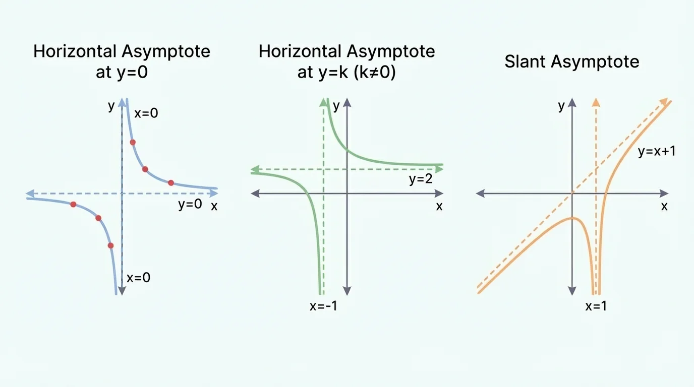
When \(x\) becomes very large or very negative, a rational function often settles into a simpler pattern. This long-run pattern is called end behavior, and the figure shows the most common possibilities.
[Figure 2] To determine end behavior, compare the degrees of the numerator and denominator.
If the degree of the numerator is less than the degree of the denominator, then the horizontal asymptote is \(y=0\).
If the degrees are equal, then the horizontal asymptote is the ratio of the leading coefficients. For example, if \(f(x)=\dfrac{3x^2-1}{2x^2+5x}\), then the horizontal asymptote is \(y=\dfrac{3}{2}\).
If the degree of the numerator is exactly one greater than the degree of the denominator, the graph has a slant asymptote. You find it by polynomial division.
There are also cases where the numerator degree is more than one greater than the denominator degree. Then the graph may approach a polynomial curve, not just a line. In many high school examples, the main focus is on horizontal and slant asymptotes.
Why leading terms control end behavior
Far from the origin, the highest-power terms dominate the value of each polynomial. That means a function like \(\dfrac{2x^3-5x+1}{x^3+4}\) behaves much like \(\dfrac{2x^3}{x^3}=2\) for very large \(|x|\). This is why comparing degrees and leading coefficients works so well.
End behavior does not tell you everything about the graph, but it tells you what happens on the far left and far right, which is essential for an accurate sketch.
For a rational function in factorable form, a reliable method is to work in an organized order.
Step 1: Factor the numerator and denominator completely.
Step 2: Identify any common factors. These create holes when canceled.
Step 3: Find zeros from the simplified numerator, making sure the denominator is not zero there.
Step 4: Find vertical asymptotes from the simplified denominator.
Step 5: Find the \(y\)-intercept, if it exists, by substituting \(x=0\).
Step 6: Determine horizontal or slant asymptotes from the degrees.
Step 7: Check the sign of the function in intervals around zeros and asymptotes to see whether branches are above or below the \(x\)-axis.
Step 8: Sketch the graph, showing intercepts, holes, asymptotes, and end behavior.
Consider \(f(x)=\dfrac{(x-1)(x+2)}{(x-3)(x+1)}\).
Worked example: graph a rational function with no common factors
Step 1: Find the zeros.
The numerator is zero when \((x-1)(x+2)=0\), so \(x=1\) and \(x=-2\). Since neither value makes the denominator zero, the graph has \(x\)-intercepts at \((1,0)\) and \((-2,0)\).
Step 2: Find the vertical asymptotes.
The denominator is zero when \((x-3)(x+1)=0\), so \(x=3\) and \(x=-1\). These are vertical asymptotes.
Step 3: Find the \(y\)-intercept.
Substitute \(x=0\): \(f(0)=\dfrac{(-1)(2)}{(-3)(1)}=\dfrac{2}{3}\). So the \(y\)-intercept is \((0,\dfrac{2}{3})\).
Step 4: Determine the horizontal asymptote.
Both numerator and denominator have degree \(2\). The leading coefficients are both \(1\), so the horizontal asymptote is
\(y=1\)
Step 5: Describe end behavior.
As \(x\to \infty\) and as \(x\to -\infty\), \(f(x)\to 1\). The graph approaches \(y=1\) on both ends.
These features give a strong hand sketch: two vertical asymptotes at \(x=-1\) and \(x=3\), two \(x\)-intercepts, one \(y\)-intercept, and branches approaching \(y=1\).
Notice how much information comes from factoring alone. You do not need a long table of values to start the graph accurately.
Now consider \(g(x)=\dfrac{(x-2)(x+3)}{(x-2)(x-1)}\). This example shows why simplifying carefully matters.
Worked example: identifying a hole
Step 1: Simplify the expression.
The common factor \((x-2)\) cancels, so for graphing behavior away from the undefined point, \(g(x)\) behaves like \(\dfrac{x+3}{x-1}\).
Step 2: Identify the hole.
Because \((x-2)\) was canceled, the original function is undefined at \(x=2\). Find the missing \(y\)-value using the simplified form: \(\dfrac{2+3}{2-1}=5\). So there is a hole at \((2,5)\).
Step 3: Find zeros and asymptotes.
The simplified numerator is zero at \(x=-3\), so the graph has an \(x\)-intercept at \((-3,0)\). The simplified denominator is zero at \(x=1\), so there is a vertical asymptote at \(x=1\).
Step 4: Find the horizontal asymptote.
The simplified function has equal degrees in numerator and denominator, with leading coefficient ratio \(\dfrac{1}{1}=1\). Therefore,
\(y=1\)
Step 5: Find the \(y\)-intercept.
Using the original function at \(x=0\): \(g(0)=\dfrac{(-2)(3)}{(-2)(-1)}=-3\). So the \(y\)-intercept is \((0,-3)\).
The graph looks like the graph of \(\dfrac{x+3}{x-1}\), except for the missing point at \((2,5)\).
This is one of the easiest places to make a mistake. A canceled factor does not disappear from the domain; it only changes the kind of discontinuity.
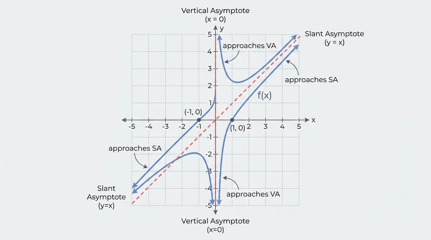
Some rational functions do not level off to a horizontal line. Instead, they approach a diagonal line. The figure helps connect the algebra to the graph, making this situation easier to understand visually.
[Figure 3] Consider \(h(x)=\dfrac{x^2+1}{x-1}\).
Worked example: finding a slant asymptote
Step 1: Identify vertical asymptotes and zeros.
The denominator is zero at \(x=1\), so there is a vertical asymptote at \(x=1\). The numerator \(x^2+1\) has no real zeros, so there are no real \(x\)-intercepts.
Step 2: Find the \(y\)-intercept.
Substitute \(x=0\): \(h(0)=\dfrac{0^2+1}{0-1}=-1\). So the \(y\)-intercept is \((0,-1)\).
Step 3: Use polynomial division.
Divide \(x^2+1\) by \(x-1\): \(x^2+1=(x-1)(x+1)+2\). Therefore,
\[h(x)=x+1+\frac{2}{x-1}\]
Step 4: Identify the slant asymptote.
Since \(\dfrac{2}{x-1}\to 0\) as \(|x|\to \infty\), the graph approaches
\(y=x+1\)
Step 5: Describe end behavior.
As \(x\to \infty\), \(h(x)\) gets closer to the line \(y=x+1\) from above. As \(x\to -\infty\), it gets closer to the same line from below.
The graph has one vertical asymptote, no real zeros, one \(y\)-intercept, and a slant asymptote of \(y=x+1\).
Later, when you compare this to horizontal-asymptote cases, the difference becomes clear: the branches do not flatten out; they align with a diagonal trend.
To sketch more accurately, check whether the function is positive or negative in each interval determined by zeros and vertical asymptotes. Pick test values.
For example, if \(f(x)=\dfrac{x+2}{x-3}\), the critical values are \(x=-2\) and \(x=3\). Test the intervals \(( -\infty,-2)\), \((-2,3)\), and \((3,\infty)\).
If \(x=-3\), then \(f(-3)=\dfrac{1}{6}>0\). If \(x=0\), then \(f(0)=\dfrac{2}{-3}<0\). If \(x=4\), then \(f(4)=6>0\).
So the graph is above the \(x\)-axis on the first and third intervals, and below it on the middle interval. Near the vertical asymptote \(x=3\), one side goes to \(-\infty\) and the other to \(+\infty\). This local behavior helps you place each branch correctly.
Engineers and scientists often care more about what happens near a restricted value than about the exact value there. Rational functions are useful because their asymptotes highlight those critical thresholds clearly.
A graph can cross a horizontal asymptote, but it cannot intersect a vertical asymptote because the function is undefined at that \(x\)-value. That distinction matters.
Rational functions appear whenever one varying quantity is divided by another. Average cost is a common example. If a company has a fixed cost of $5,000 and a variable cost of $8 per item, then the average cost per item for producing \(x\) items is
\[A(x)=\frac{5000+8x}{x}=\frac{5000}{x}+8\]
As \(x\) grows, \(\dfrac{5000}{x}\) becomes very small, so the average cost approaches \(8\). That means the graph has horizontal asymptote \(y=8\). The end behavior tells you what happens in large-scale production.
Another example comes from travel. If you drive a fixed distance of \(240\) miles at speed \(v\), the travel time is \(t(v)=\dfrac{240}{v}\). This is a rational function. As speed increases, time decreases, but speed cannot be \(0\), so \(v=0\) is not allowed. The graph reflects a real restriction in the situation.
In physics, inverse relationships such as intensity and distance can also create rational models. Interpreting the graph means understanding restrictions, impossible values, and long-run behavior, not just plotting points. This is exactly why recognizing asymptotes and zeros is so useful, as we saw earlier when comparing end-behavior patterns.
One common mistake is assuming every denominator zero creates a vertical asymptote. If the factor cancels, the result is a hole instead.
Another mistake is finding zeros from the original numerator without checking whether that factor also appears in the denominator. A canceled factor does not produce an \(x\)-intercept.
Students also sometimes think a horizontal asymptote is a ceiling the graph cannot cross. That is false. A rational graph may cross a horizontal asymptote and still approach it for large \(|x|\).
Finally, do not ignore the simplified form when determining asymptotes and zeros, but do not ignore the original form when determining the domain. You need both views.
| Feature | How to find it | What it means on the graph |
|---|---|---|
| Zero | Set simplified numerator equal to \(0\) | Usually an \(x\)-intercept |
| Vertical asymptote | Set simplified denominator equal to \(0\) | Graph grows without bound near that \(x\)-value |
| Hole | Look for canceled factors | Missing point on the curve |
| Horizontal asymptote | Compare degrees and leading coefficients | End behavior approaches a constant \(y\)-value |
| Slant asymptote | Use division when numerator degree is one greater | End behavior approaches a line |
Table 1. Main graph features of rational functions and how to identify them from symbolic form.
When a rational function is given in a suitable factored form, the graph becomes much easier to interpret. Factoring is not just an algebra skill; it is a way to read the structure of the graph directly.