A city can grow richer by clearing more forest, pumping more groundwater, or catching more fish—at least for a while. Then the same decisions can trigger soil loss, polluted water, shrinking habitats, and a food system that becomes less reliable. That is the central challenge of sustainability: choices that look successful in the short term can weaken the natural systems that human societies depend on in the long term. A computational simulation helps us see those hidden connections before they become real-world crises.
In Earth and Space Science, sustainability is not just about "using fewer resources." It is about understanding how Earth systems, living systems, and human systems interact. Forests regulate water flow, wetlands filter pollutants, pollinators support crops, and biodiversity helps ecosystems recover from stress. When people manage natural resources responsibly, they are also managing the conditions that support agriculture, health, economic stability, and the future size and well-being of human populations.
This topic focuses on creating or using a simplified model, such as a spreadsheet or a provided multi-parameter program, to represent those interactions. The goal is not to build a highly advanced computer program. Instead, the goal is to organize variables, apply simple update rules, and observe how a system changes from one time step to the next.
Natural resources include materials and environmental conditions that humans use, such as fresh water, soil, forests, fisheries, minerals, sunlight, and fertile land. Some resources renew quickly, some renew slowly, and some are effectively nonrenewable on human time scales.
Human population sustainability depends on whether enough food, water, energy, and space remain available over time. If a population uses resources faster than they can recover, the system becomes unstable. People may still meet their needs for a short period, but eventually shortages, environmental damage, or economic disruption appear.
Biodiversity matters because ecosystems are not just scenery. They perform work. A biodiverse forest stores carbon, holds soil in place, slows runoff, supports insects and birds, and creates habitat for countless organisms. A river system with many species often responds better to disturbance than one that has already been simplified or damaged. Biodiversity supports ecosystem services, which are benefits humans receive from functioning ecosystems.
Sustainability is the ability of a system to continue over time without exhausting the resources or environmental conditions it depends on.
Ecosystem services are the benefits humans receive from healthy ecosystems, including pollination, water purification, soil formation, climate regulation, and food production.
Because these ideas are connected, scientists and planners often study them together. A farming region, for example, is not only about crop yield. It is also about groundwater recharge, soil fertility, habitat area, species diversity, flood control, and the number of people the land can support year after year.
A computational simulation is a model that uses calculations to show how a system may change over time under different conditions. In a classroom setting, that often means a spreadsheet with rows representing years and columns representing variables such as population size, water supply, forest cover, or biodiversity level.
Each variable changes according to rules. For instance, a resource stock might increase by regeneration and decrease by human use. A simple update equation for resource stock can be written as \[R_{t+1} = R_t + G - U\] where \(R_t\) is the current resource amount, \(G\) is resource regeneration during that time step, and \(U\) is resource use. If a forest starts with \(R_t = 1{,}000\) units, the resource stock increases by \(G = 80\) units per year, and humans remove \(U = 120\) units, then \(R_{t+1} = 1{,}000 + 80 - 120 = 960\). The stock declines.
Simulations become more realistic when they include more than one variable. Biodiversity may decrease when habitat shrinks. Food production may drop if soil quality falls. Human population support may depend on both resource supply and biodiversity. Even with only a few variables, a simulation can reveal patterns that are hard to notice in words alone.
Remember that a model is a simplified representation of a real system. Models are useful because they focus attention on important relationships, but they always leave out some details.
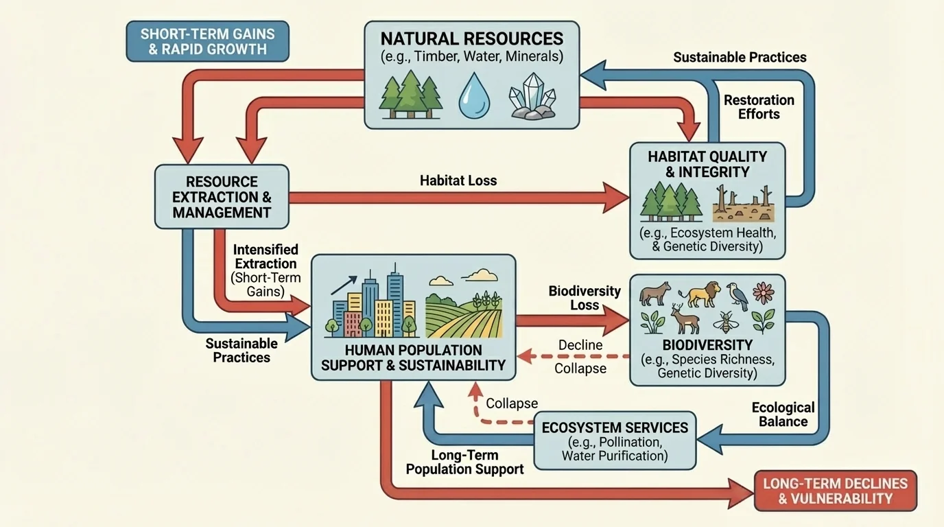
In this topic, the acceptable level of modeling stays simple and clear. As [Figure 1] shows, a provided multi-parameter program or a spreadsheet calculation is enough. The important scientific thinking is choosing meaningful variables, explaining the assumptions, and interpreting the results carefully.
These systems are linked by feedback loops. A change in one part of the system can spread through several others. For example, increasing logging may raise short-term income and land available for farming, but it may also reduce habitat, lower biodiversity, increase erosion, and damage water quality. Those changes can later reduce crop productivity and make the region less able to support its population.
Some feedbacks are reinforcing. If soil degrades, crop yield may fall. To compensate, people may clear even more land, which causes more erosion and further soil degradation. Other feedbacks are stabilizing. If a fishery is managed with catch limits, fish populations can recover, which helps maintain food supply over many years.
One important idea is carrying capacity. In ecology, this is the maximum population size an environment can support over time. In human systems, carrying capacity is more flexible because technology, trade, and management can increase or decrease how many people a region can support. However, carrying capacity is not unlimited. If water tables drop, fisheries collapse, or soils lose fertility, the effective carrying capacity falls.
A simple way to represent this in a model is to connect population support to resource availability and biodiversity. For example, suppose a region's population support capacity is estimated by \[K = 0.5R + 200B\] where \(K\) is the number of people the system can support, \(R\) is a scaled resource stock, and \(B\) is a biodiversity index between \(0\) and \(1\). If \(R = 800\) and \(B = 0.9\), then \(K = 0.5(800) + 200(0.9) = 400 + 180 = 580\). If biodiversity drops to \(0.4\), then \(K = 400 + 80 = 480\). The same amount of raw resource supports fewer people because ecosystem quality has declined.
That is why biodiversity is not a side issue. As we saw in [Figure 1], it helps determine whether ecosystems remain productive, stable, and resilient enough to support human needs.
As [Figure 2] illustrates, to create a useful simulation, start by defining the system boundary. Are you modeling a forest region, a river basin, a fishery, or an agricultural valley? Then choose a small set of variables that capture the key relationships.
A spreadsheet model works well because each row can represent one year, one season, or another time step. Columns might include time, resource stock, regeneration rate, extraction, habitat quality, biodiversity index, technology efficiency, and population support. The calculations in one row feed into the next row.
Typical update rules are simple. Resource stock may equal previous stock plus regeneration minus use. Biodiversity may decline when habitat quality falls and recover slowly when habitat improves. Population may rise when support capacity is high and level off or decline when support capacity is low.
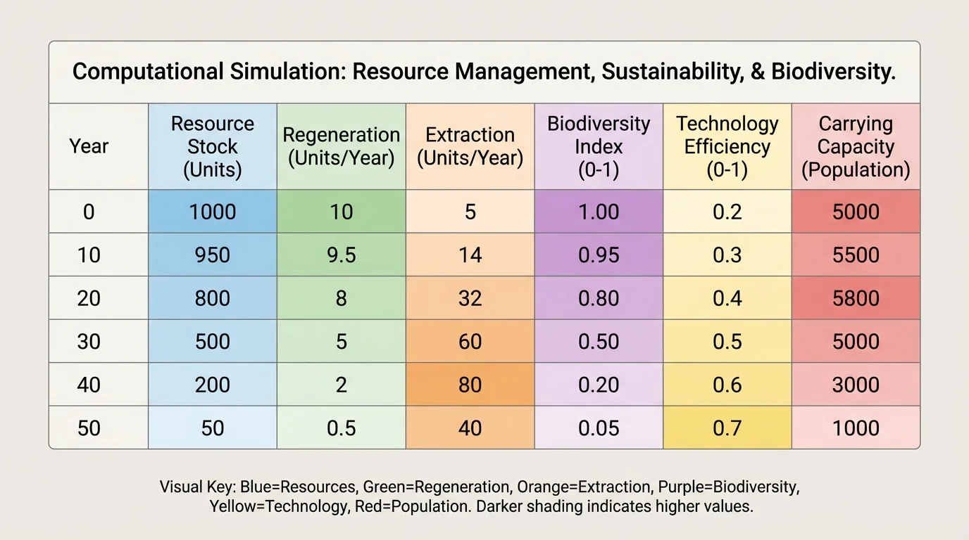
Assumptions must be clear. If you assume that biodiversity responds immediately to habitat loss, say so. If you assume regeneration is constant, say so. In real systems, regeneration often depends on climate, pollution, and species interactions. But a simplified model may treat it as a constant so that the major relationships remain understandable.
Choosing parameters wisely
Parameters are fixed values used in a model, such as a regeneration rate of \(80\) units per year or a biodiversity decline of \(0.02\) per year when habitat quality is poor. Good parameters are plausible, consistent, and clearly explained. A simulation does not become better just because it has more numbers; it becomes better when the numbers represent meaningful science.
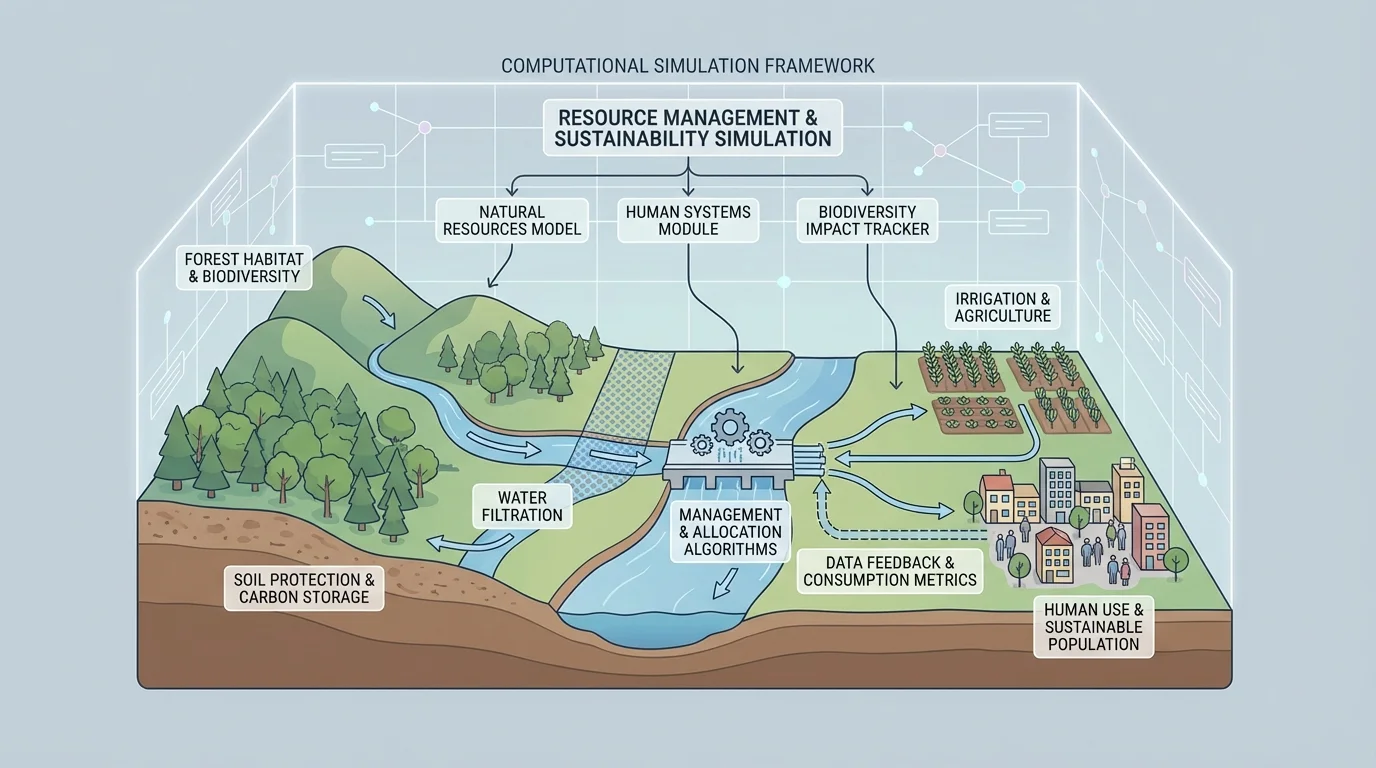
As [Figure 3] shows, it is also useful to distinguish between variables people can control and variables they cannot. Extraction rate, recycling rate, irrigation efficiency, and protected habitat area are management choices. Rainfall, drought, wildfire, or disease outbreak may be external factors that affect the system but are not directly controlled by decision-makers.
Consider a region with upland forest, a river, farmland, and a town. The forest supplies timber, protects soil, stores water, and provides habitat. The river supplies irrigation water and drinking water. Farms provide food. The town depends on all three.
Suppose the simulation includes four main variables: forest cover \(F\), water quality \(W\), biodiversity index \(B\), and population support \(P_s\). Forest cover is measured in percentage points from \(0\) to \(100\). Water quality and biodiversity are measured on a scale from \(0\) to \(1\). Population support estimates how many people the system can sustainably support.
One possible set of simplified rules is:
Forest next year: \(F_{t+1} = F_t + r - h\), where \(r\) is reforestation and natural regrowth, and \(h\) is forest removed.
Water quality next year: \(W_{t+1} = W_t + 0.002(F_t - 50) - 0.01p\), where \(p\) represents pollution pressure. This means water quality improves when forest cover is above \(50\) and worsens with pollution.
Biodiversity next year: \(B_{t+1} = B_t + 0.01(W_t - 0.5) + 0.003(F_t - 50)\). Higher forest cover and cleaner water help biodiversity.
Population support: \(P_s = 300 + 4F + 200W + 150B\).
Worked simulation step
Suppose the starting values are \(F = 70\), \(W = 0.80\), and \(B = 0.75\). During one year, reforestation is \(r = 2\), forest harvest is \(h = 5\), and pollution pressure is \(p = 3\).
Step 1: Update forest cover.
\(F_{t+1} = 70 + 2 - 5 = 67\).
Step 2: Update water quality.
\(W_{t+1} = 0.80 + 0.002(70 - 50) - 0.01(3) = 0.80 + 0.04 - 0.03 = 0.81\).
Step 3: Update biodiversity.
Using the previous year's \(W_t = 0.80\) and \(F_t = 70\), \(B_{t+1} = 0.75 + 0.01(0.80 - 0.5) + 0.003(70 - 50) = 0.75 + 0.003 + 0.06 = 0.813\).
Step 4: Estimate population support.
\(P_s = 300 + 4(67) + 200(0.81) + 150(0.813)\).
\(P_s = 300 + 268 + 162 + 121.95 = 851.95\).
The model predicts support for about 852 people at this stage.
This is not a perfect description of reality. But it clearly shows how one management choice—harvesting more forest—can influence water, biodiversity, and the number of people the system can support. A stronger harvest might raise short-term timber supply while lowering long-term support.
Because all four variables are connected, the region behaves like a system, not a set of isolated parts. The landscape shown in [Figure 3] makes that visible: forest loss affects the river, the river affects farms and the town, and habitat quality affects biodiversity across the whole watershed.
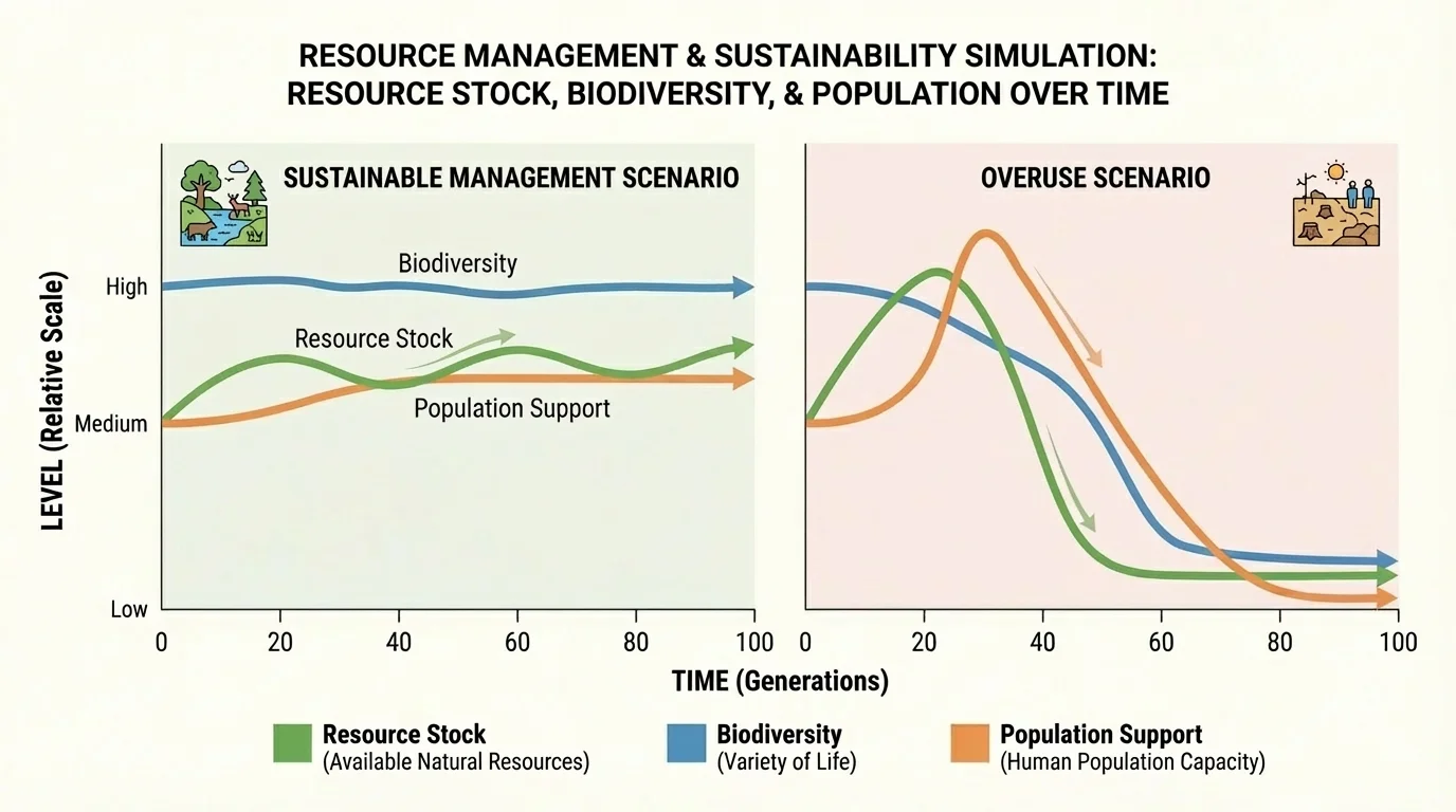
As [Figure 4] illustrates, once the spreadsheet runs for many time steps, the output usually appears as rows of values and line graphs. Scenario graphs are especially powerful because they let you compare what happens under different choices such as high extraction, moderate extraction, or conservation-focused management.
As [Figure 4] illustrates, look for trends rather than single-year changes. A small annual decline can become a major loss over decades. Also watch for thresholds. Some systems seem stable until a variable crosses a critical level, after which decline accelerates. A lake can absorb some nutrient pollution, but beyond a certain point water quality may drop rapidly.
Another important pattern is lag time. Biodiversity may not respond instantly to habitat loss. A forest bird population may continue for several years after fragmentation, then decline later when nesting sites and food webs have been disrupted. That means short-term stability in a graph does not always mean long-term sustainability.
A useful comparison table can help organize outcomes from different scenarios.
| Scenario | Extraction Level | Habitat Protection | Likely Resource Trend | Likely Biodiversity Trend | Long-Term Population Support |
|---|---|---|---|---|---|
| Overuse | High | Low | Declines quickly | Drops | Falls after short-term rise |
| Balanced use | Moderate | Moderate | Stable or slow decline | Mostly stable | More stable |
| Restoration-focused | Lower | High | Recovers gradually | Improves | May rise after delay |
Table 1. Comparison of likely long-term outcomes under different resource management strategies.
When interpreting a graph, ask: Which variable changes first? Which variable responds later? Does the system recover if management improves, or has it crossed a threshold that makes recovery slow? The curves in [Figure 4] help answer those questions by showing not just whether a system changes, but how it changes over time.
Many real ecosystems can appear productive while they are quietly losing resilience. For a time, fertilizer, irrigation, or intensive harvesting can hide environmental decline, but the system may become more vulnerable to drought, pests, or disease.
Technology can shift outcomes in a simulation because it changes how efficiently resources are used or how damage is reduced. Drip irrigation reduces water loss. Wastewater treatment improves water quality. Selective logging can lower habitat damage compared with clear-cutting. Renewable energy can reduce pollution from fossil fuel use.
A simple efficiency factor can be included in the model. If water demand is \(D\) and irrigation efficiency is \(e\), actual withdrawal might be represented as \(U = D(1 - e)\). If demand is \(100\) units and efficiency is \(0.20\), then \(U = 100(1 - 0.20) = 80\). If improved technology raises efficiency to \(0.45\), then \(U = 100(1 - 0.45) = 55\). The same agricultural output now requires less water extraction.
Technology does not automatically solve sustainability problems. Sometimes greater efficiency lowers cost and leads to more total use, a pattern sometimes called a rebound effect. A simulation can test this by increasing efficiency but also increasing demand. If demand rises too much, total resource use may still climb.
Technology comparison example
A region needs the equivalent of \(120\) units of irrigation service.
Step 1: Compute water withdrawal with low efficiency.
If \(e = 0.25\), then \(U = 120(1 - 0.25) = 90\).
Step 2: Compute water withdrawal with improved efficiency.
If \(e = 0.50\), then \(U = 120(1 - 0.50) = 60\).
Step 3: Interpret the effect.
The improved system reduces withdrawal by \(90 - 60 = 30\) units. In a larger simulation, that lower withdrawal can help maintain river flow, protect wetland habitat, and support biodiversity.
Management choices such as harvest quotas, protected areas, pollution limits, and restoration programs can be added to the same model. In that way, a simulation becomes a tool for comparing policies instead of just describing damage.
No simulation is the real world. A spreadsheet may treat biodiversity as a single number, but actual biodiversity includes genes, species, populations, and ecosystems. It may combine all pollution into one variable, even though different pollutants affect organisms differently. These simplifications are acceptable if they are acknowledged.
Parameters and equations should be chosen because they reflect sensible science, not because they produce a desired answer. If two groups use different assumptions, they may get different results. That is not failure; it is a reminder to examine the assumptions carefully.
Ethically, models should not be used to hide trade-offs. A project that increases short-term income but destroys critical habitat may still look attractive if biodiversity is ignored. Responsible modeling includes environmental costs and long-term consequences.
"We do not inherit the Earth from our ancestors; we borrow it from our children."
— Proverb
That idea fits simulation work perfectly. A good model asks not only, "What happens next year?" but also, "What kind of system are we leaving for the future?"
Governments and scientists use simulations to help manage fisheries, forests, groundwater basins, and urban growth. In a fishery, managers may compare catch limits to estimate how fish populations and harvests change over time. In a forested watershed, planners may compare logging strategies to see how timber production, stream quality, and habitat are affected.
Water managers use similar models to explore drought response. If groundwater is pumped faster than recharge, water levels fall. If wetlands shrink, biodiversity may decline and flood protection may weaken. A simulation can show which combinations of conservation, technology, and restoration keep the system within sustainable limits.
Urban planners also depend on this kind of thinking. Expanding roads and housing can support a growing population, but if growth replaces wetlands, fragments forests, and increases runoff, the city may become less resilient to heat, flooding, and water shortages. Sustainability requires managing both the built environment and the natural systems that support it.
The most powerful lesson from simulation is that environmental decisions are rarely isolated. Resource management, biodiversity, and human population sustainability form one connected problem. A simplified computational model helps make those links visible, measurable, and open to comparison.