A conservation decision can affect thousands of organisms before anyone realizes whether it worked. If a highway cuts through a forest, if farms increase pesticide use, or if a fishery allows one more year of heavy harvesting, the consequences may unfold over many generations. That is why scientists often turn to simulations: they let us test possible solutions before entire populations or ecosystems pay the price.
Biodiversity includes variation at several levels: genetic diversity within a species, the number of species in an area, and the variety of ecosystems across a region. When biodiversity decreases, ecosystems often become less stable, less productive, and less able to recover from disturbances such as drought, disease, or fire.
Testing solutions directly in nature is important, but it can also be slow, expensive, and ethically difficult. A simulation allows scientists to ask questions such as: What happens to pollinator populations if pesticide use drops by half? How much does a wildlife corridor increase survival? Will a marine reserve help fish populations recover in ten years or only in fifty? Instead of waiting decades for every answer, researchers build models that estimate what may happen under different conditions.
In high school biology, a simulation is best understood as a simplified, rule-based representation of a real system. It does not copy nature perfectly. Instead, it captures the most important relationships so that changes in one factor can be tested against changes in another.
Simulation is a model that imitates how a real system changes over time. Mitigation means reducing the severity of a harmful impact. Biodiversity refers to the variety of life at genetic, species, and ecosystem levels.
Simulations are especially valuable in ecology because ecosystems are complex. A change in one species may affect a predator, a pollinator, a decomposer, and a food source all at once. This means good environmental decisions often depend on understanding interactions, not just isolated facts.
As [Figure 1] shows, human actions alter ecosystems in many ways. A road can split one habitat into smaller fragments. Fertilizer runoff can trigger algal blooms that lower oxygen in water. Global trade can introduce invasive species. Overfishing can remove top predators and change food webs. Each of these changes can lower survival, reduce reproduction, or shrink the area where species can live.
Habitat fragmentation happens when a large, continuous habitat is broken into smaller pieces. Even if some habitat remains, species may no longer move easily between patches. That matters because movement affects access to food, mates, shelter, and new territory. Fragmentation can also reduce gene flow, the movement of genes between populations through reproduction, which may increase the risk of inbreeding and lower resilience.
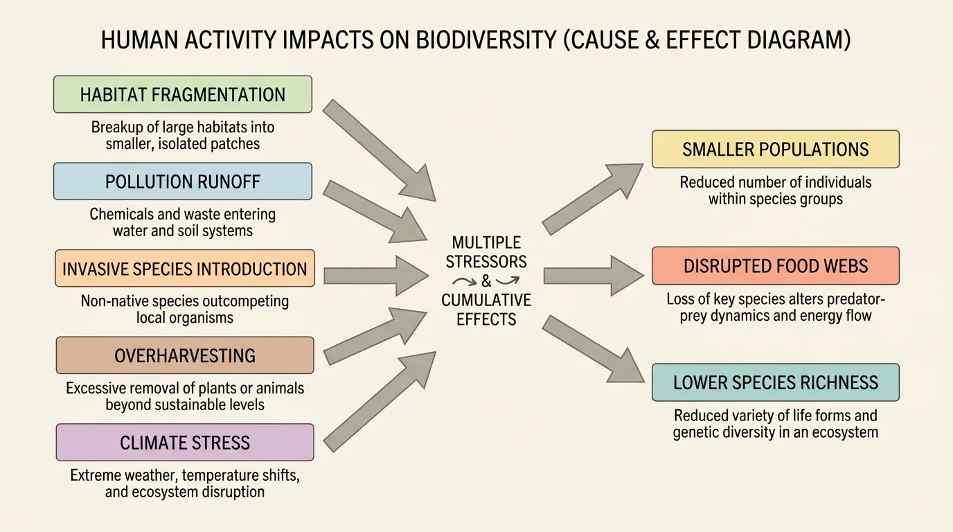
Pollution can act directly or indirectly. For example, excess nitrogen and phosphorus entering waterways can stimulate rapid growth of algae. When the algae die and decompose, oxygen levels drop. Fish and invertebrates may then die or move away. A simulation of this system might track nutrient input, algal growth, dissolved oxygen, and fish survival over time.
Invasive species can outcompete native species, spread disease, or alter habitats. Climate change shifts temperature and rainfall patterns, causing some species to migrate, decline, or lose synchrony with seasonal resources. A flower may bloom earlier while its pollinator still emerges on the old schedule. These mismatches show why biodiversity problems often involve timing as well as population size.
Human impacts rarely act alone. A fragmented landscape may also experience warming temperatures and increased pollution. This is one reason simulations are powerful: they can combine several stressors in one system instead of examining each one separately.
Some species can remain present in a habitat for years after conditions worsen, even though their populations are no longer truly sustainable. Ecologists sometimes call this an "extinction debt," meaning the full impact of habitat loss may appear later than the original disturbance.
That delayed response makes conservation challenging. If a population appears stable today, it may still be heading toward decline because reproduction has already fallen below replacement level.
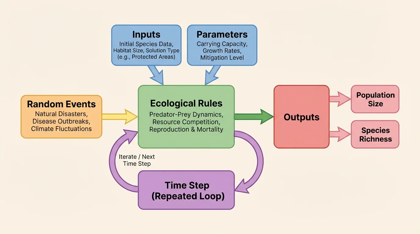
A strong ecological simulation has a clear structure. First come the variables, the factors that can change, such as population size, habitat area, temperature, or pollution level. Next come the rules or relationships connecting those variables. For instance, if habitat quality decreases, mortality may increase and reproduction may decrease.
Simulations also use parameters, which are fixed values chosen for a particular run of the model, such as birth rate, death rate, carrying capacity, or migration rate. Some models include random events because real ecosystems are not perfectly predictable. Drought, wildfire, disease outbreaks, and harsh winters can all affect outcomes.
Many ecological simulations update conditions in repeated time steps. At each step, the model calculates a new population size or biodiversity measure. A simple population update can be represented as
\[N_{t+1} = N_t + B - D + I - E\]
where population at the next time step depends on the current population, births, deaths, immigration, and emigration. Suppose a bird population begins with \(N_t = 200\), with \(B = 30\), \(D = 20\), \(I = 10\), and \(E = 5\). Then \(N_{t+1} = 200 + 30 - 20 + 10 - 5 = 215\). Even a simple equation like this can help show how a corridor, a hunting restriction, or habitat restoration changes outcomes.
A useful simulation needs more than equations. It also needs good assumptions. If a model assumes all habitat patches are identical when they are not, its predictions may be misleading. If it ignores predators or seasonal breeding cycles, it may miss a key driver of change.
Outputs from simulations may include total population size, number of species, extinction risk, average genetic diversity, or the percent of habitat occupied. Scientists compare outputs across different scenarios to evaluate possible solutions.
Models are simplified, not fake
A simulation becomes scientifically valuable when its simplifications are thoughtful. The goal is not to include every detail in an ecosystem. The goal is to include the factors that most strongly affect the question being studied. A simple model can be more useful than an overly complicated one if it clearly tests the right mechanism.
This is why a good simulation begins with a well-defined question. "Will restoring \(20\%\) of wetland area increase amphibian survival?" is a better modeling question than "What happens in wetlands?" The first question tells you what variable to change and what output to measure.
A mitigation solution is a strategy meant to reduce environmental harm. In biodiversity studies, this might include restoring habitat, connecting separated habitats with wildlife corridors, setting catch limits in fisheries, reducing pesticide use, controlling invasive species, planting native vegetation, or creating protected areas.
The best solution to model depends on the problem. If fragmentation is the main threat, a corridor or underpass might be the right intervention. If nutrient pollution is driving fish deaths, the solution may be reducing runoff from farms. If pollinators are declining, a useful strategy could be lowering pesticide exposure while increasing flowering habitat.
To choose a testable solution, identify the target species or community, the harmful human activity, and the measurable outcome. For example, "Build a corridor between two forest patches to increase movement of lynx and reduce local extinction risk" is specific enough to simulate. "Help wildlife" is not.
Case study setup: Pollinator-friendly farming
A farming region has fewer native bees after years of heavy pesticide use and removal of flowering field margins. A simulation might compare two scenarios: current farming practices and a mitigation plan with reduced pesticide use plus restored flower strips.
Step 1: Choose variables
Possible variables include bee population size, flower abundance, pesticide exposure, and crop pollination rate.
Step 2: Set relationships
If flower abundance increases, bee survival and reproduction may increase. If pesticide exposure increases, mortality may rise.
Step 3: Compare outputs
The model can track whether bee populations stay above a minimum viable level over multiple seasons.
Notice that this simulation tests a solution, not just a problem. That distinction matters because conservation science aims to guide action.
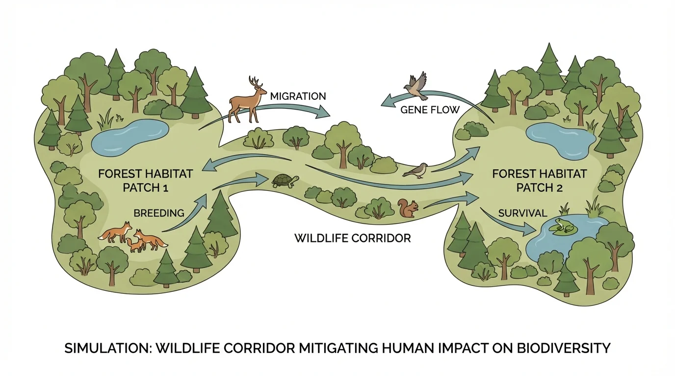
When scientists build a model, they first identify the system parts and how those parts interact. A corridor model provides a good template: two habitat patches, a population in each patch, movement between patches, and survival or reproduction influenced by habitat quality. If the corridor is added, migration may increase, which can raise gene flow and reduce local extinction risk.
One way to represent limited growth is with a carrying capacity model. Carrying capacity is the largest population an environment can support over time. A common form is
\[N_{t+1} = N_t + rN_t\left(1 - \frac{N_t}{K}\right)\]
where \(r\) is growth rate and \(K\) is carrying capacity. If \(N_t = 50\), \(r = 0.2\), and \(K = 100\), then the change is \(0.2 \cdot 50 \cdot (1 - 50/100) = 10 \cdot 0.5 = 5\), so \(N_{t+1} = 55\). If restoring habitat increases \(K\) from \(100\) to \(140\), the same population can grow more strongly because the environment supports more individuals.
In a corridor simulation, migration might be added as a fraction of the population moving each time step. If one isolated patch has migration rate \(m = 0.01\) and the corridor raises it to \(m = 0.08\), the model can compare whether higher movement lowers extinction risk over many years.
Building the model also means deciding what level of detail to use. A simple model may represent one species only. A more advanced model may include predators, competitors, or plants that provide food. Neither is automatically better. The right choice depends on whether the added detail improves the answer to the question.
Data sources matter. Parameters can come from field surveys, published studies, satellite imagery, camera traps, fish counts, or genetic analyses. If scientists know average juvenile survival, annual rainfall, or nesting success, they can use those values to make the model more realistic.
Earlier work in ecology shows that population size alone does not tell the whole story. Age structure, access to habitat, food supply, competition, and climate conditions all affect whether a population is truly stable.
A simulation may also include biodiversity metrics beyond one population. Species richness is simply the number of species present. A model might estimate how many bird species remain in a wetland under different restoration plans. If one plan maintains \(18\) species while another maintains \(25\), the second may better protect community diversity.
The first version of a model is rarely the final one. Revising matters because ecological systems are messy, and revision is a cycle rather than a single correction. Scientists compare model outputs to observed data, identify mismatches, adjust assumptions or parameters, and rerun the model.
Calibration means adjusting model parameters so outputs fit known data reasonably well. Validation means checking whether the model also predicts data that were not used to tune it. For example, a fish population model might be calibrated using counts from the first five years and validated against counts from the next three years.
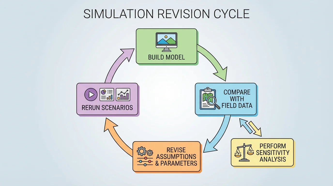
Another important revision tool is sensitivity analysis. This means changing one input at a time to see which variables most affect the output. If a corridor model changes dramatically when juvenile survival shifts slightly, but barely changes when adult migration changes, then juvenile survival is a high-sensitivity parameter.
Consider a quick example. Suppose a restored wetland simulation predicts frog population size after one year. With juvenile survival \(s = 0.30\), the model predicts \(120\) frogs. With \(s = 0.40\), it predicts \(150\) frogs. That \(0.10\) increase in survival leads to \(30\) more frogs, suggesting the model is quite sensitive to that factor. A revised model might therefore focus on better field estimates for juvenile survival.
Worked revision example: Marine reserve simulation
A model predicts reef fish recovery after part of a coastline becomes a no-take zone, but the predicted recovery is faster than what field surveys show.
Step 1: Compare model output to observed data
The model predicts \(800\) fish after \(5\) years, but field data show only \(620\).
Step 2: Look for missing factors
The original model included reproduction and fishing mortality but ignored coral bleaching and storm damage.
Step 3: Revise assumptions
Add periodic habitat loss events and lower juvenile survival during bleaching years.
Step 4: Rerun and test
If the revised output matches field trends more closely, the model becomes more credible for decision-making.
Revision is not a sign that the first model failed. It is a normal part of science. Good models improve through testing.
Simulation output is useful only if it is interpreted carefully. A claim should connect the tested solution to the evidence. For example: "Adding a corridor reduced local extinction risk in the model because migration increased and isolated populations no longer declined as quickly." That claim is stronger than simply saying the corridor "helped."
Most simulations compare at least two scenarios: a baseline with current conditions and one or more mitigation scenarios. If a baseline predicts a steady decline from \(300\) to \(120\) individuals over \(20\) years, while a restoration scenario stabilizes the population near \(260\), the restoration appears beneficial. If a second scenario raises the population to \(290\) but costs far more or harms another species, decision-makers must weigh trade-offs.
Uncertainty always remains. Random events, incomplete data, and simplified assumptions mean model outputs are estimates, not guarantees. Simulation results depend on the structure of the model and the chosen input values, and revision and sensitivity analysis help scientists judge how trustworthy the conclusions are.
Scientists also look for patterns across repeated runs. If a model includes randomness, one run may not be enough. A corridor may reduce extinction risk in \(85\%\) of runs rather than all runs. That still supports the solution, but it also communicates uncertainty honestly.
Wildlife corridor planning is one of the clearest real-world uses of ecological simulation. In regions where roads divide forests, scientists model animal movement between habitat patches. The corridor system shown earlier in [Figure 3] captures the basic logic: increasing movement can connect isolated populations, improve gene flow, and reduce the risk that one small local population disappears permanently.
Marine reserves provide another example. Simulations can test whether limiting fishing in a protected area allows fish populations to recover enough to spill into nearby waters. A model may track adult survival, reproduction, larval dispersal, and fishing pressure outside the reserve. These models help balance biodiversity protection with food production and local livelihoods.
On farms, simulation can guide pollinator protection by comparing different levels of pesticide reduction, flower-strip restoration, and crop rotation. In freshwater systems, models can test whether wetland restoration lowers nutrient pollution and improves survival of fish, amphibians, and aquatic plants.
"All models are wrong, but some are useful."
— George Box
This statement does not dismiss modeling. It reminds us that no model is perfect, but a carefully built and tested model can still provide powerful guidance.
Simulations should support decisions, not replace observations in nature. A model may overlook cultural values, economic constraints, rare events, or species interactions that were never measured. It may predict average outcomes well but miss unusual years when drought or disease changes everything.
That is why conservation scientists combine simulation with field studies, experiments, monitoring, and local knowledge. The cause-and-effect relationships shown in [Figure 1] help identify causes of biodiversity loss, while the model structure shown in [Figure 2] helps test possible solutions. Together, they make biodiversity science more predictive and more useful for real choices.
When you create or revise a simulation, you are doing more than running numbers. You are identifying relationships in living systems, testing how human actions change those systems, and using evidence to judge whether a solution can protect the diversity of life.