A change in one part of Earth can ripple across the whole planet. When sea ice melts in the Arctic, the ocean absorbs more solar energy. That extra heat affects air temperature, ocean circulation, ecosystems, and even weather patterns far away. Earth is not a set of isolated parts; it is a connected system. As shown in [Figure 1], scientists use computational representations to make those connections visible and measurable through linked spheres and flows.
To understand climate change, it is not enough to know that the atmosphere is warming. We also need to understand how the atmosphere interacts with oceans, land, living things, and ice. A computational representation is a scientific way of organizing these interactions using variables, relationships, and rules based on evidence. In this topic, the goal is not to run a climate model yourself. Instead, the focus is on using the published results of scientific models to understand how Earth systems affect one another and how human actions are changing those relationships.
Earth scientists often divide the planet into major subsystems. These include the atmosphere, the layer of gases surrounding Earth; the hydrosphere, which includes liquid water; the geosphere, the solid Earth; the biosphere, all living organisms; and the cryosphere, which includes frozen water such as glaciers, sea ice, and snow. Although these categories are useful, the boundaries between them are constantly crossed by moving matter and energy.
For example, water evaporates from the ocean into the atmosphere, condenses into clouds, falls as precipitation, moves across land, and returns to rivers and oceans. Carbon also moves among systems through the carbon cycle. Plants take in carbon from the atmosphere in the form of greenhouse gases such as \(\textrm{CO}_2\), animals and microbes return carbon to the atmosphere, and oceans absorb and release carbon as conditions change. These pathways are dynamic, not fixed.
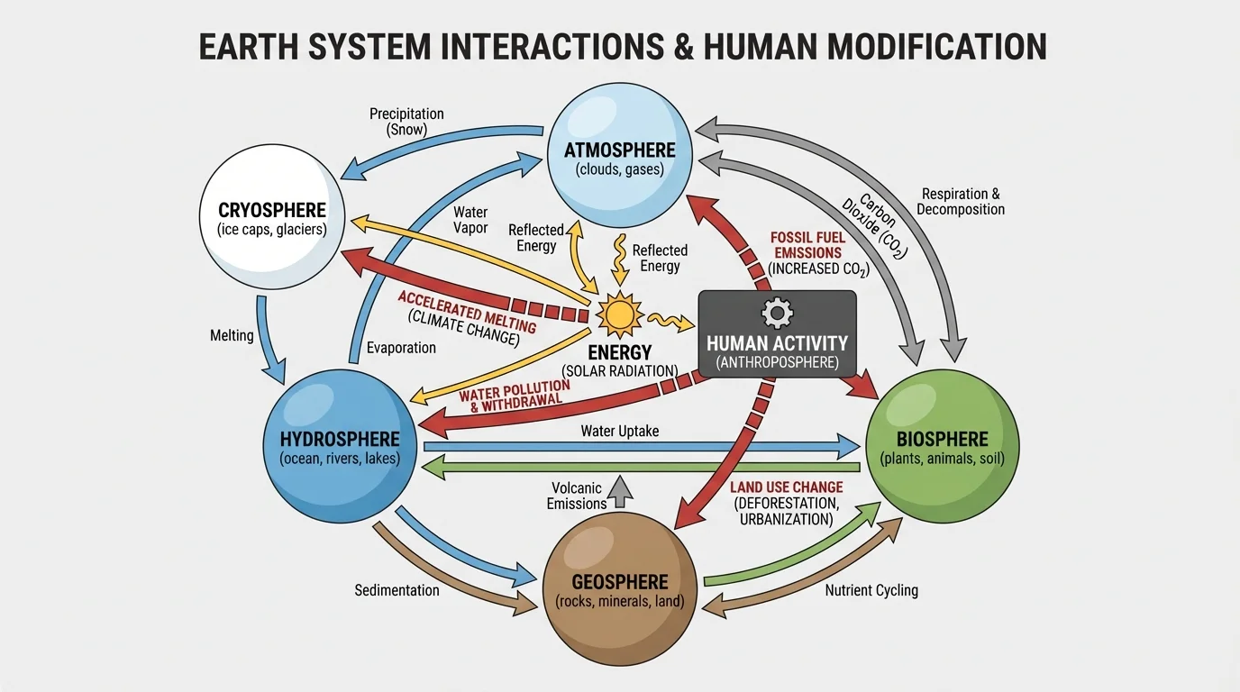
Energy also links Earth systems. Incoming solar radiation warms Earth's surface. Some energy is reflected back to space, some is absorbed by land and water, and some is re-radiated as infrared energy. Gases such as \(\textrm{CO}_2\), methane, and water vapor absorb and re-emit some of that infrared energy, warming the lower atmosphere. This process is called the greenhouse effect.
The interactions among these systems are sometimes gradual and sometimes rapid. A volcanic eruption can send particles into the atmosphere within hours, affecting sunlight and temperature. By contrast, the growth of an ice sheet or the buildup of carbon in the deep ocean can occur over centuries to millennia. Computational representations are especially valuable because they help scientists track changes operating on different timescales at the same time.
Computational representation is a scientific model that uses variables, data, and relationships to describe how parts of a system interact and change over time. In Earth science, these representations can connect atmospheric temperature, ocean currents, ice cover, vegetation, and other factors in one framework.
A useful way to think about Earth systems is as a network. Each sphere is like a node, and arrows between nodes represent exchanges of matter or energy. No system stands alone. If the atmosphere changes, the ocean may respond. If the biosphere changes, the carbon balance may shift. If the cryosphere shrinks, the energy balance may change.
As shown in [Figure 2], scientists build computational representations by identifying key variables and the relationships among them through inputs, processes, and outputs. A model does not include every tiny detail of the real world. Instead, it includes the most important features needed to answer a question, such as how temperature, precipitation, or sea level may change under different conditions.
In a climate model, variables might include atmospheric \(\textrm{CO}_2\) concentration, average surface temperature, cloud cover, sea ice area, ocean heat content, or vegetation cover. A relationship describes how one variable affects another. For instance, if atmospheric \(\textrm{CO}_2\) increases, more infrared energy is trapped, which tends to increase temperature. If temperature increases, ice may melt. If ice melts, Earth reflects less sunlight, which can lead to additional warming.
That last kind of response is called a feedback. A positive feedback increases the original change, while a negative feedback reduces it. One important positive feedback is the ice-albedo effect. Since bright ice reflects more sunlight than darker ocean water or land, melting ice reduces reflectivity and increases absorption of solar energy. A negative feedback example can occur when warmer conditions increase plant growth in some regions, allowing more carbon to be stored in biomass, though this effect has limits.
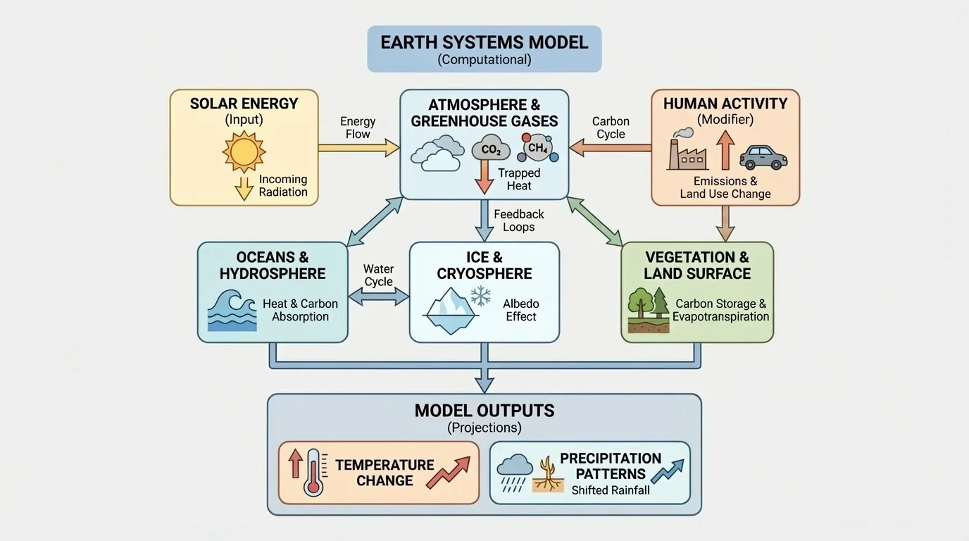
Computational representations also use inputs and outputs. Inputs may include solar energy, volcanic particles, land cover, and greenhouse gas concentrations. Outputs may include projected global temperature, rainfall patterns, ice loss, or sea-level rise. Many published climate studies compare outputs under different scenarios, which are scientifically reasoned descriptions of possible future conditions based on assumptions about emissions and land use.
Scientists test these models by comparing their results with observations. If a model can reproduce past climate patterns reasonably well, confidence in its usefulness increases. This does not mean the model is perfect. It means the model captures important relationships in the Earth system. Modern climate models improve by using better observations, more detailed physics, and stronger understanding of interactions among atmosphere, ocean, land, and ice.
Earlier Earth science topics introduced the idea that matter cycles and energy flows through natural systems. Computational representations build on that idea by turning system interactions into organized, evidence-based relationships that can be analyzed over time.
A simple numerical relationship can help illustrate forcing and response. Suppose Earth receives an average incoming solar energy of \(340 \textrm{ W/m}^2\), and increased greenhouse gases reduce outgoing energy by about \(2 \textrm{ W/m}^2\). That imbalance may seem small, but spread across the entire planet and sustained over years, it leads to significant heat gain, especially in the oceans. Climate models track many such imbalances together rather than treating them one at a time.
One essential relationship is between the atmosphere and hydrosphere. The ocean stores a huge amount of thermal energy because water has a high specific heat. This means oceans warm more slowly than land, but they can store and transport enormous quantities of heat. Ocean currents redistribute energy from equatorial regions toward higher latitudes, influencing climate patterns.
Another key relationship is between the atmosphere and biosphere. Plants remove \(\textrm{CO}_2\) from the atmosphere during photosynthesis and convert it into organic matter. A simplified equation for photosynthesis is \[6\textrm{CO}_2 + 6\textrm{H}_2\textrm{O} \rightarrow \textrm{C}_6\textrm{H}_{12}\textrm{O}_6 + 6\textrm{O}_2\] This process links atmospheric chemistry to ecosystems, soil carbon, and food webs. If large forests are removed, the atmosphere may gain more \(\textrm{CO}_2\), and local water cycling can also change because forests release water vapor through transpiration.
The cryosphere strongly affects the atmosphere and hydrosphere through reflectivity and freshwater input. Snow and ice have high albedo, meaning they reflect a large fraction of incoming sunlight. Dark ocean water has much lower albedo. If sea ice decreases, more solar energy is absorbed, which can warm surface waters further. Meltwater from glaciers and ice sheets also adds freshwater to the ocean, affecting salinity and circulation.
The geosphere matters too. Weathering of rocks can remove carbon from the atmosphere over long timescales. Volcanic eruptions can inject ash and sulfur-containing particles into the atmosphere, temporarily cooling the planet by reflecting sunlight. Soil, which forms at the boundary of the geosphere and biosphere, stores carbon and water and influences plant growth, runoff, and erosion.
Earth systems are linked by cycles and feedbacks. A cycle moves matter, such as water or carbon, through different parts of Earth. A feedback changes the strength of a process after an initial change occurs. Climate behavior emerges from many cycles and feedbacks operating together, not from one single cause acting alone.
Published climate model results often show these links together. For example, a warming atmosphere increases evaporation. More water vapor can intensify some storms because warmer air can hold more moisture. A common approximation is that the atmosphere can hold about \(7\%\) more water vapor for each \(1^{\circ}\textrm{C}\) of warming. If a region's air mass could hold \(100\) units of water vapor before warming, then after \(1^{\circ}\textrm{C}\) warming it could hold about \(107\) units. That does not guarantee every storm becomes stronger, but it helps explain why heavy rainfall risk can increase.
As shown in [Figure 3], human activity changes Earth systems not only by adding new materials but also by altering the links among systems through the carbon cycle and energy balance. The most important modern example is the large-scale release of greenhouse gases from burning coal, oil, and natural gas. These fuels store carbon that was locked underground for millions of years. When burned, they release \(\textrm{CO}_2\) into the atmosphere much faster than natural long-term geologic processes would.
A simplified combustion example is the burning of methane: \[\textrm{CH}_4 + 2\textrm{O}_2 \rightarrow \textrm{CO}_2 + 2\textrm{H}_2\textrm{O}\] This reaction shows that carbon in fuel becomes atmospheric \(\textrm{CO}_2\). If human emissions increase atmospheric greenhouse gas concentration, the greenhouse effect strengthens. That changes temperature, precipitation, ocean heat storage, ice cover, and ecosystem conditions.
Deforestation also modifies system relationships. Trees store carbon, cool the environment through transpiration, and influence local rainfall. Removing forests can reduce carbon uptake, increase erosion, warm land surfaces, and alter regional weather. In the Amazon, for example, scientists study whether enough forest loss could weaken moisture recycling and shift parts of the region toward drier conditions.
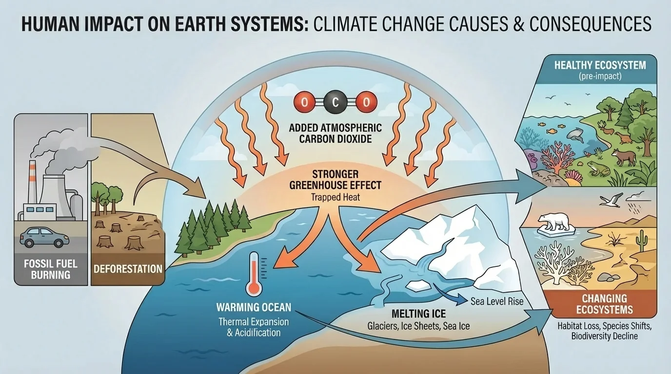
Agriculture changes Earth systems in several ways. Livestock and rice cultivation release methane, a powerful greenhouse gas. Fertilizer use can increase nitrous oxide emissions. Land conversion changes albedo, soil moisture, and runoff. Urbanization creates heat islands because dark surfaces such as asphalt absorb and retain heat differently than vegetation-covered land. Impermeable surfaces also change how water moves, increasing runoff and flood risk during intense rain.
Human-produced aerosols add another layer of complexity. Some aerosols reflect sunlight and can have a cooling effect. Others absorb energy or affect cloud formation. Because different human influences can push climate in different directions, computational representations are essential for estimating their combined effects. As shown earlier in [Figure 2], climate models organize many interacting processes in one system rather than treating them separately.
Case study: rising atmospheric \(\textrm{CO}_2\) and system-wide change
Step 1: Human activities increase emissions
Burning fossil fuels and clearing forests add more \(\textrm{CO}_2\) to the atmosphere.
Step 2: The atmosphere retains more heat
More greenhouse gases strengthen the greenhouse effect and raise average temperature.
Step 3: Other systems respond
Oceans absorb much of the added heat, land ice melts, ecosystems shift, and precipitation patterns change.
Step 4: Feedbacks can intensify changes
Reduced ice cover lowers albedo, and thawing permafrost can release additional greenhouse gases.
This chain shows why climate change is an Earth-systems problem, not only an atmospheric one.
Another major human impact is ocean acidification. The ocean absorbs some atmospheric \(\textrm{CO}_2\). When \(\textrm{CO}_2\) dissolves in seawater, it forms carbonic acid and changes ocean chemistry, making it harder for some organisms to build shells and skeletons from calcium carbonate. This links atmospheric emissions directly to marine ecosystems.
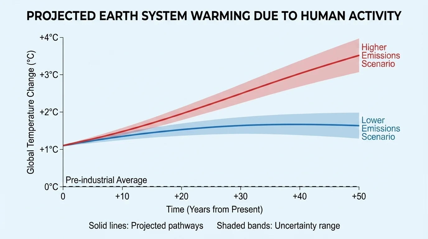
As shown in [Figure 4], scientists often present published model results as graphs, maps, and comparison tables. A temperature projection graph may include several lines representing different emissions scenarios. Lower-emissions pathways usually show less warming over time than higher-emissions pathways. The message is not that the future is random; it is that future conditions depend partly on human choices.
Another common feature is an uncertainty range, often shown as a shaded band around a line. This does not mean scientists know nothing. It means there is a range of plausible outcomes based on natural variability, different model structures, and uncertainty in future human behavior. Even with uncertainty, broad patterns such as long-term warming from increased greenhouse gases are strongly supported by evidence.
Scientists also use ensemble modeling, which means comparing many model runs or many models together. If multiple models with different details point toward similar trends, confidence in those trends increases. An ensemble average can reduce the effect of unusual behavior from any single model.
Maps of model output may show that warming is not equal everywhere. Land often warms faster than ocean, and the Arctic warms especially quickly. Precipitation projections also vary by region. Some places are expected to experience heavier rainfall events, while others face increased drought risk. To read these maps well, students should look for patterns, compare regions, and note whether results are consistent across models.
Published model results can also show time delays. Because the ocean stores heat, some climate responses continue even after emissions slow. This is one reason why sea level can keep rising for a long time. Thermal expansion means that as water warms, its volume increases. If a sample of seawater expands from \(1.000\) liter to \(1.003\) liters when warmed, that is a \(0.3\%\) increase in volume. Across the global ocean, a small fractional expansion contributes significantly to sea-level rise.
| Published model output | What it helps explain | Example interpretation |
|---|---|---|
| Global temperature graph | Long-term warming trend | Higher emissions produce greater warming over time |
| Regional precipitation map | Where wet and dry conditions may shift | Some regions show increased heavy rainfall risk |
| Sea-level projection graph | Future coastal risk | Rise continues because of thermal expansion and land ice melt |
| Sea ice trend graph | Cryosphere response | Declining ice cover reduces albedo and affects ecosystems |
Table 1. Common types of published climate model results and what students can infer from them.
The ocean has absorbed most of the excess heat trapped by greenhouse gases. This is why global warming is not just an air-temperature story; it is also a story about changing ocean conditions.
Scenario-based graphs are especially useful because they connect human choices to projected outcomes. They do not predict one guaranteed future. They compare scientifically modeled futures under different assumptions.
The Arctic is one of the clearest examples of interacting Earth systems. Air temperatures there are rising faster than the global average, a pattern often called Arctic amplification. Reduced sea ice lowers albedo, allowing darker ocean water to absorb more solar energy. This adds heat to the local system, which promotes further melting. The cryosphere, hydrosphere, and atmosphere are tightly linked here.
Coastal communities experience another Earth-systems consequence: sea-level rise. Two major causes are thermal expansion of warming seawater and the addition of water from melting land ice. Higher sea level increases the reach of storm surge and raises flood risk during high tides. Here, atmospheric warming affects the ocean and cryosphere, and the results directly affect human infrastructure.
In many regions, changing precipitation patterns influence agriculture, freshwater supply, and wildfire risk. Hotter conditions can dry soils more quickly, stressing crops and vegetation. In some places, reduced snowpack lowers summer water availability. In others, warmer air contributes to heavier downpours. The exact pattern differs by location, which is why regional published model results are so important.
Real-world interpretation example
Step 1: Read the trend
A published graph shows that a region's average temperature rises by about \(2^{\circ}\textrm{C}\) over several decades under a higher-emissions scenario.
Step 2: Connect systems
Higher temperature can increase evaporation, lower soil moisture, and lengthen dry seasons.
Step 3: Infer impacts
The region may face more drought stress, greater wildfire risk, and changing habitat conditions.
This is how scientists and decision-makers use published model results: not as exact daily forecasts, but as evidence-based guides to system-level change.
Ocean acidification provides a strong example of chemistry linked to biology. As atmospheric \(\textrm{CO}_2\) rises, more of it dissolves into seawater. This can lower pH and reduce carbonate availability, affecting corals, shellfish, and plankton. Since many marine food webs depend on these organisms, the effects can spread through the biosphere. Human emissions change the atmosphere, which changes ocean chemistry, which then changes living systems.
Climate models improve as scientists gather more accurate observations from satellites, weather stations, ocean buoys, ice cores, and field measurements. Better observations help scientists refine model equations and test whether results match the real world. Advances in computing also allow models to use smaller grid sizes, which improves representation of coastlines, storms, topography, and ocean circulation.
Improvement does not mean earlier models were useless. In fact, many older projections correctly identified the direction of major climate trends, especially long-term warming under rising greenhouse gas concentrations. Newer models tend to represent more processes in greater detail and provide better regional information.
These models matter because societies make decisions in the present that shape future risk. City planners use sea-level projections to design coastal infrastructure. Farmers and water managers use precipitation projections to prepare for drought or flooding. Public health systems study heat projections to protect vulnerable populations. Insurance, energy, transportation, and conservation planning all depend on understanding likely future conditions.
"The climate system is an interconnected whole."
— A central idea in Earth system science
One of the most important scientific lessons is that Earth system change is rarely linear and isolated. A rise in atmospheric \(\textrm{CO}_2\) does not only increase air temperature. It changes ocean heat, ice cover, biological productivity, weather extremes, and chemical conditions in water and soil. That is why computational representations are so valuable: they reveal relationships that are too interconnected to track by intuition alone.
By connecting evidence, published model outputs, and system interactions, Earth science helps us understand both natural processes and human influence. The major goal is not to memorize every variable in a model. It is to understand that Earth's atmosphere, oceans, land, ice, and life are linked, and that human activity is now a powerful force modifying those links.