When a password fails because two characters are swapped, or when the probability of getting a certain poker hand depends on exactly which cards are chosen, probability is not just about guessing what seems likely. In many situations, you can calculate it exactly by counting how many outcomes are possible and how many of them are favorable.
Many probability problems are built on a uniform probability model. That means every outcome in the sample space is equally likely. In that setting, probability can often be found with a simple idea:
\[P(\textrm{event}) = \frac{\textrm{number of favorable outcomes}}{\textrm{number of possible outcomes}}\]
The challenge is usually not the fraction itself. The challenge is counting correctly. If you count too few outcomes, your probability will be too large. If you count the same outcome more than once, your probability will be wrong in a different way. That is why permutations and combinations are essential tools.
Permutation means an arrangement in which order matters.
Combination means a selection in which order does not matter.
Compound event is an event made of two or more simpler events, such as getting a heart and a face card, or choosing a captain or a goalie.
Before using formulas, it helps to understand the structure of the situation. Ask two questions: How many choices are made? and Does the order of those choices matter?
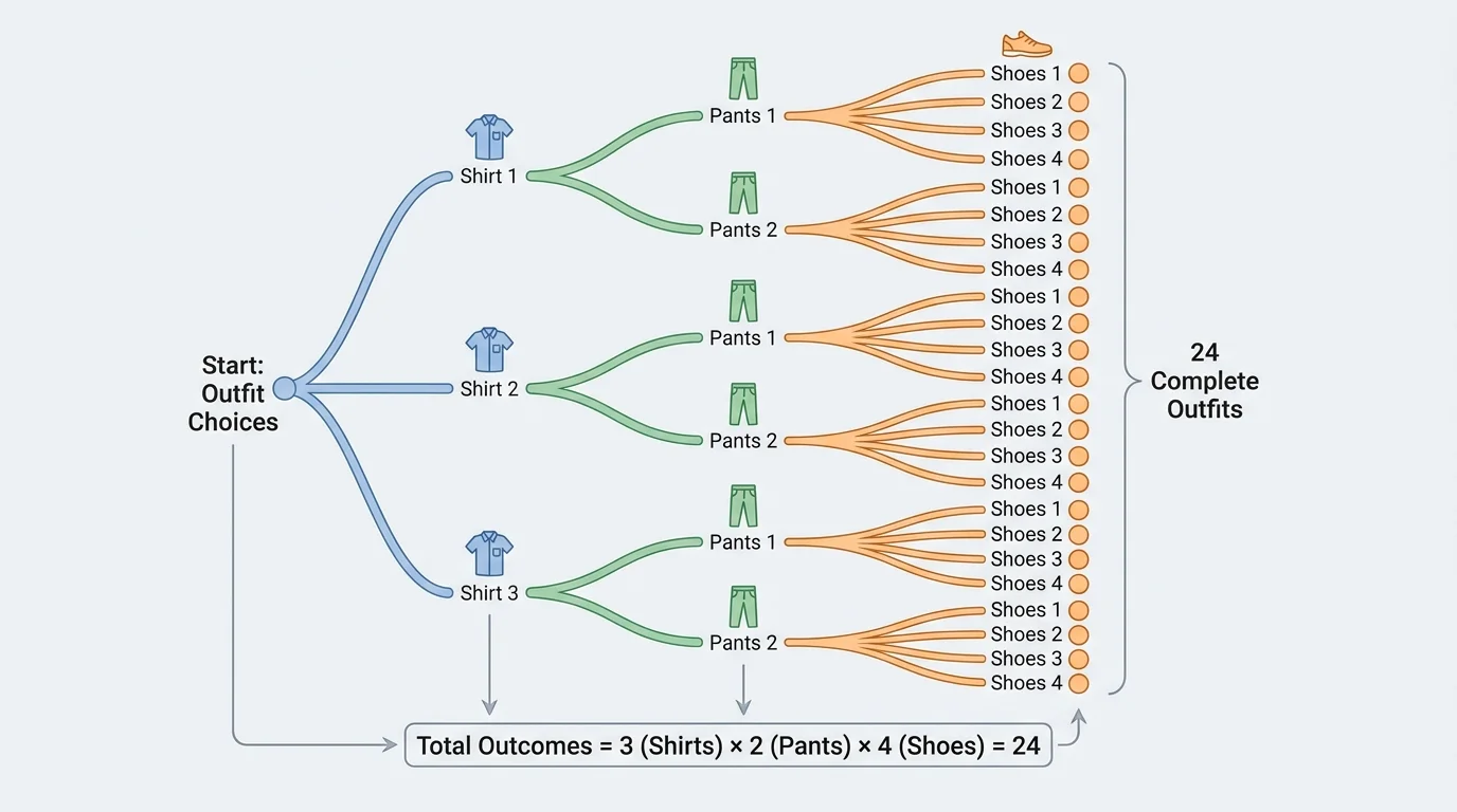
One of the most useful tools in counting is the multiplication principle. If one step can happen in \(a\) ways and a second step can happen in \(b\) ways, then the two-step process can happen in \(ab\) ways. For longer processes, multiply all the numbers of choices together. This kind of multi-stage counting is easy to visualize with branching, as [Figure 1] shows.
For example, if a student can choose from \(3\) shirts, \(2\) pairs of pants, and \(4\) pairs of shoes, then the total number of outfits is \(3 \cdot 2 \cdot 4 = 24\).
Another important counting tool is the factorial. For a positive integer \(n\), the factorial is written \(n!\) and means the product of all positive integers from \(n\) down to \(1\):
\[n! = n(n-1)(n-2)\cdots 2\cdot 1\]
For instance, \(5! = 5 \cdot 4 \cdot 3 \cdot 2 \cdot 1 = 120\). Factorials appear naturally when we arrange objects in order. If there are \(5\) different books and you want to place them on a shelf, there are \(120\) possible orders.
The same idea from [Figure 1] applies to probability. If an event happens in stages, you can often count all possible outcomes by multiplying the options at each stage, then count the favorable ones the same way.
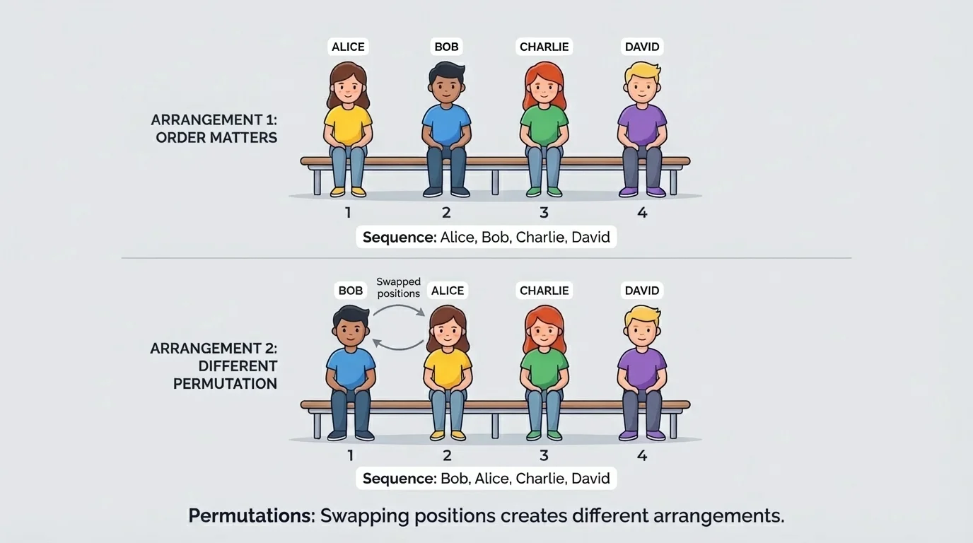
A permutation counts arrangements when order matters. If \(n\) distinct objects are arranged using all of them, the number of permutations is \(n!\). Different orders create different outcomes, as [Figure 2] illustrates.
If only \(r\) objects are chosen from \(n\) distinct objects and arranged, the number of permutations is
\[{}_nP_r = \frac{n!}{(n-r)!}\]
Why does this formula work? The first position has \(n\) choices, the second has \(n-1\), and so on until \(r\) positions are filled. So the product is \(n(n-1)(n-2)\cdots(n-r+1)\), which is equivalent to \(\dfrac{n!}{(n-r)!}\).
Suppose \(4\) students sit in \(4\) chairs in a row. The orders \(ABCD\) and \(BACD\) are different because the positions changed. That is why this is a permutation situation.
Restrictions are common in permutation problems. For example, if \(5\) runners are placed in first through third place, there are \({}_5P_3 = \dfrac{5!}{2!} = 60\) possible outcomes. But if one runner must be first, then only the remaining \(4\) runners compete for second and third, giving \({}_4P_2 = 12\) outcomes.
Secure systems depend on the fact that the number of possible arrangements grows extremely fast. Even adding one more character to a code can multiply the number of possibilities dramatically.
When repeated objects appear, the counting changes because some arrangements look the same. For example, the letters in the word LEVEL are not all distinct. Counting repeated-letter permutations is an advanced variation, but the key idea is to divide by the number of repeated rearrangements that do not create new outcomes.
A combination counts selections when order does not matter. If you are choosing a committee of \(3\) students from \(10\), the group \({A,B,C}\) is the same committee as \({B,C,A}\). Since those are not different outcomes, this is not a permutation.
The formula for combinations is
\[{}_nC_r = \binom{n}{r} = \frac{n!}{r!(n-r)!}\]
This formula comes from taking the number of permutations and dividing by \(r!\), because each selected group of \(r\) people can be arranged in \(r!\) ways that all represent the same group.
For example, the number of ways to choose \(3\) students from \(10\) is
\[\binom{10}{3} = \frac{10!}{3!7!} = 120\]
Notice how different that is from \({}_{10}P_3 = 720\). The permutation count is larger because it treats different orders as different outcomes.
| Situation | Order matters? | Method |
|---|---|---|
| Assign president, vice president, secretary | Yes | Permutation |
| Choose a 3-person committee | No | Combination |
| Create a 4-digit code | Yes | Permutation or multiplication principle |
| Select 5 cards from a deck | No | Combination |
Table 1. Comparison of situations where order matters and where it does not.
Once you can count outcomes, probability follows from the ratio of favorable outcomes to total outcomes. In a uniform probability model, this is often written as
\[P(E) = \frac{n(E)}{n(S)}\]
Here, \(n(E)\) is the number of outcomes in the event and \(n(S)\) is the number of outcomes in the sample space.
Suppose a committee of \(2\) students is chosen from \(8\) students. What is the probability that both chosen students are seniors if \(3\) of the \(8\) students are seniors? The total number of committees is \(\binom{8}{2} = 28\). The favorable committees come from choosing \(2\) of the \(3\) seniors: \(\binom{3}{2} = 3\). So the probability is \(\dfrac{3}{28}\).
Counting creates the sample space
Probability rules depend on knowing what outcomes are possible. Permutations and combinations do not replace probability rules; they help build the sample space so those rules can be applied correctly. In many real problems, the main work is identifying what should be counted.
This approach is especially useful for compound events. Instead of listing every possible outcome by hand, you count them efficiently.
A compound event may involve an intersection, a union, or a complement. The language of the problem gives clues.
"And" usually refers to the intersection of events. For events \(A\) and \(B\), \(A \cap B\) means outcomes that are in both events.
"Or" usually refers to the union of events. For events \(A\) and \(B\), \(A \cup B\) means outcomes that are in at least one of the events.
The general addition rule is
\[P(A \cup B) = P(A) + P(B) - P(A \cap B)\]
The subtraction matters because outcomes in both events would otherwise be counted twice.
The complement of an event \(A\), written \(A^c\), contains all outcomes not in \(A\). Its probability is
\[P(A^c) = 1 - P(A)\]
Complements are especially helpful when "at least one" appears. Often it is easier to compute the probability of "none" and subtract from \(1\).
Solved example 1: Using combinations for a card probability
Five cards are chosen from a standard \(52\)-card deck. What is the probability that all \(5\) cards are hearts?
Step 1: Count all possible \(5\)-card hands.
The total number of hands is \(\binom{52}{5}\).
Step 2: Count the favorable hands.
There are \(13\) hearts, and we need to choose \(5\) of them, so the number of favorable hands is \(\binom{13}{5}\).
Step 3: Form the probability.
\[P(\textrm{all hearts}) = \frac{\binom{13}{5}}{\binom{52}{5}} = \frac{1287}{2{,}598{,}960}\]
This probability is very small because only a tiny fraction of all \(5\)-card hands contain only hearts.
The reason combinations are used here is that a hand of cards is a selection, not an arrangement. The order in which the cards are dealt does not matter for the final hand.
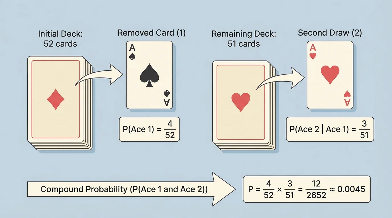
Sometimes one event changes the sample space for the next event. That is the idea of conditional probability. If the first event affects what can happen next, then the second probability must be computed from a smaller or different set of outcomes, as [Figure 3] shows with card draws without replacement.
The formula is
\[P(A \mid B) = \frac{P(A \cap B)}{P(B)}\]
This means the probability of \(A\) given \(B\) is the probability that both happen, divided by the probability that \(B\) happens.
If two events are independent events, then one does not affect the probability of the other. In that case, \(P(A \mid B) = P(A)\), and the multiplication rule becomes
\[P(A \cap B) = P(A)P(B)\]
But many counting problems are not independent. Drawing cards without replacement, selecting students for a team, and choosing parts from a box all change the next step.
Solved example 2: Conditional probability with two card draws
Two cards are drawn from a standard deck without replacement. What is the probability that both cards are aces?
Step 1: Find the probability of an ace on the first draw.
There are \(4\) aces in \(52\) cards, so \(P(\textrm{first ace}) = \dfrac{4}{52}\).
Step 2: Adjust the sample space for the second draw.
After drawing one ace, there are \(3\) aces left in \(51\) cards, so \(P(\textrm{second ace} \mid \textrm{first ace}) = \dfrac{3}{51}\).
Step 3: Multiply the probabilities.
\[P(\textrm{both aces}) = \frac{4}{52} \cdot \frac{3}{51} = \frac{1}{221}\]
This is a compound event using an intersection: first ace and second ace.
The changing sample space in [Figure 3] is exactly why the two probabilities are not the same. The first draw is based on \(52\) cards, but the second is based on \(51\).
Solved example 3: Committee selection
A club has \(6\) juniors and \(4\) seniors. A \(3\)-student committee is chosen at random. What is the probability that the committee has exactly \(2\) juniors and \(1\) senior?
Step 1: Count all possible committees.
The total number of \(3\)-student committees from \(10\) students is \(\binom{10}{3} = 120\).
Step 2: Count favorable committees.
Choose \(2\) of the \(6\) juniors and \(1\) of the \(4\) seniors:
\[\binom{6}{2}\binom{4}{1} = 15 \cdot 4 = 60\]
Step 3: Compute the probability.
\[P(\textrm{exactly 2 juniors and 1 senior}) = \frac{60}{120} = \frac{1}{2}\]
This type of problem is common: count total groups, then count the groups that match the condition.
Notice how the multiplication principle works inside the favorable count. First choose the juniors, then choose the senior. Because these are separate stages in the counting process, the numbers multiply.
Solved example 4: Password arrangement
A school website uses a \(4\)-letter code made from \(6\) different letters, with no repetition. What is the probability that a randomly generated code begins with \(A\)?
Step 1: Count all possible codes.
Since order matters and there is no repetition, the total number of codes is \({}_6P_4 = \dfrac{6!}{2!} = 360\).
Step 2: Count favorable codes.
If the first letter must be \(A\), then the remaining \(3\) positions are filled from the other \(5\) letters:
\[{}_5P_3 = \frac{5!}{2!} = 60\]
Step 3: Form the probability.
\[P(\textrm{begins with } A) = \frac{60}{360} = \frac{1}{6}\]
This is a permutation problem because changing the order changes the code.
Even when formulas work well, it is smart to pause and ask whether the answer makes sense. In the password example, \(\dfrac{1}{6}\) is reasonable because there are \(6\) equally likely choices for the first letter.
These ideas appear in many fields. In cybersecurity, the number of possible PINs, passwords, or access codes depends on permutations and the multiplication principle. In medicine, probability models help estimate the chance that a test panel includes certain results. In manufacturing, selecting items from a batch helps predict the chance of drawing defective parts. In sports, probabilities can describe lineup arrangements, tournament seeding, or draft possibilities.
Suppose a quality inspector randomly selects \(3\) items from a batch of \(20\), where \(4\) are defective. The probability that at least one is defective can be found by using a complement. Instead of counting all the ways to get at least one defective, count the ways to get none defective: choose all \(3\) from the \(16\) good items. Then
\[P(\textrm{at least one defective}) = 1 - \frac{\binom{16}{3}}{\binom{20}{3}}\]
This is exactly the kind of compound event where complements save time.
If a problem feels confusing, return to two earlier ideas: identify the sample space, and decide whether outcomes are equally likely. Once those are clear, counting methods and probability rules fit together much more naturally.
Another common application is team formation. A coach may want the probability that a random \(5\)-player lineup includes at least \(2\) guards, or exactly \(1\) captain, or no first-year players. These are all counting-based probability questions.
The most common mistake is using permutations when combinations are needed, or combinations when permutations are needed. A quick test is this: if you switch the order and nothing meaningful changes, use combinations. If switching the order creates a different outcome, use permutations.
Another mistake is ignoring restrictions. If repetition is not allowed, each step has fewer choices than the one before. If repetition is allowed, the number of choices may stay the same at each step. Always read the problem carefully.
Students also sometimes forget overlap in "or" problems. If an outcome satisfies both conditions, it belongs to the intersection and must be subtracted once in the addition rule.
A good strategy is to work in this order:
First, define the sample space clearly.
Second, decide whether the event is about arrangements or selections.
Third, count the total outcomes and the favorable outcomes.
Fourth, apply probability rules such as complements, unions, intersections, or conditional probability when needed.
Used carefully, permutations and combinations turn complicated-looking probability questions into organized counting problems. That is one of the most elegant ideas in probability: when outcomes are equally likely, smart counting leads directly to exact probabilities.