A national poll can survey only a few thousand people and still make claims about millions. That sounds almost impossible at first. How can talking to a small group tell us something meaningful about everyone else? The answer lies in one of the most important ideas in statistics: if a sample is selected well, it can provide useful evidence about a population. But that evidence always comes with uncertainty, and understanding that uncertainty is exactly what good statistical reasoning is about.
[Figure 1] When statisticians want information about a large group, they usually do not measure every person or object. The entire group of interest is called the population. A smaller group chosen from it is a sample. A sample lets us learn about the population more efficiently: we collect data from a smaller group and use it to estimate a larger, unknown quantity.
If a school wants to know the average number of hours students sleep on school nights, surveying every student may take too much time. Instead, the school can select a random sample and ask those students. The result from the sample gives an estimate of the population value.
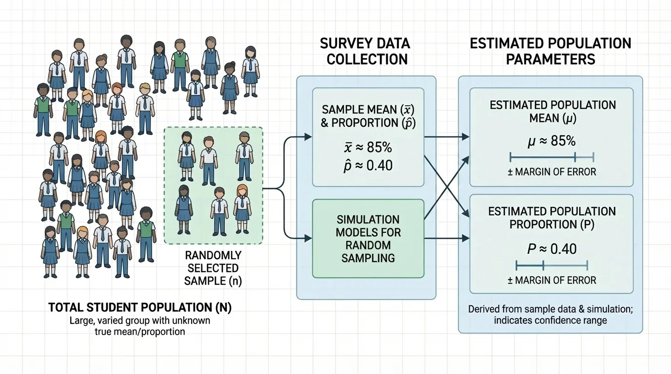
A value that describes a population is called a parameter. A value computed from a sample is called a statistic. Parameters are usually unknown. Statistics are known once we collect the sample data, and we use them to estimate parameters.
Random sampling matters because it helps produce a sample that is more representative of the population. If the sample is chosen in a biased way, the estimate can be misleading no matter how carefully we calculate.
A population is the entire group we want information about. A sample is the smaller group actually surveyed. A parameter is a numerical summary of the population, and a statistic is a numerical summary of the sample used to estimate the parameter.
A census attempts to measure every member of a population. A sample survey measures only part of the population. In many real situations, a well-designed sample survey is faster, cheaper, and still highly informative.
Two common population quantities are a population mean and a population proportion. Which one we use depends on the kind of variable being studied.
If the variable is numerical, such as height, study time, or daily screen use, we often estimate the population mean. The sample mean is written as \(\bar{x}\), and it is calculated by adding the sample values and dividing by the sample size:
\[\bar{x} = \frac{\textrm{sum of sample values}}{n}\]
If the variable is categorical, such as whether a student has a part-time job or whether a voter supports a candidate, we often estimate a population proportion. The sample proportion is written as \(\hat{p}\):
\[\hat{p} = \frac{\textrm{number with the characteristic}}{n}\]
For example, if \(84\) out of \(120\) surveyed students say they eat breakfast before school, then the sample proportion is \(\hat{p} = \dfrac{84}{120} = 0.70\). This suggests that about \(70\%\) of the population may eat breakfast before school.
From earlier work with data, a mean describes the center of numerical values, while a proportion describes the fraction or percent in a category. Statistical inference uses those familiar ideas in a new way: it uses sample results to say something about a larger population.
The sample size, written as \(n\), is crucial. Larger random samples usually produce estimates with less variability from sample to sample, although larger samples do not fix biased sampling methods.
A sample result used to estimate a population value is called a point estimate. The sample mean \(\bar{x}\) is a point estimate for the population mean \(\mu\), and the sample proportion \(\hat{p}\) is a point estimate for the population proportion \(p\).
However, a point estimate alone is not enough. Suppose two different random samples are taken from the same population. They will usually not produce exactly the same statistic. This natural change from sample to sample is called sampling variability.
Sampling variability is not a mistake. It is expected. Even with perfectly random selection, samples differ. One sample may contain slightly more athletes, another slightly more ninth graders, another slightly more students who stayed up late the night before. Those differences affect the sample statistic.
Why estimates vary
Statistics is powerful because a random sample tends to reflect the population reasonably well, but not perfectly. The estimate wanders around the true population value from sample to sample. Good inference does not pretend this wandering disappears; instead, it measures how large the wandering usually is and builds that uncertainty into the conclusion.
If the survey method systematically leaves out part of the population, then the estimate may be biased. For example, an online survey about school transportation may miss students with limited internet access at home. That problem is different from ordinary sampling variability.
[Figure 2] When news reports say a poll has a margin of error, they are describing the amount of variation expected from random sampling. A margin of error gives a range around a sample statistic that is likely to contain the true population parameter. One strong way to understand this is through simulation: repeated random samples produce a distribution of possible sample results.
Suppose the true population proportion were \(0.60\), but we do not know that. If we repeatedly take random samples of size \(100\), some sample proportions might be \(0.55\), \(0.62\), \(0.58\), \(0.64\), and so on. These values fluctuate around the true proportion because of random chance in sampling.
A simulation model imitates this process many times. We can use technology to repeatedly select random samples from a model population and record the resulting means or proportions. The spread of those simulated statistics shows how much random sampling variation is typical.
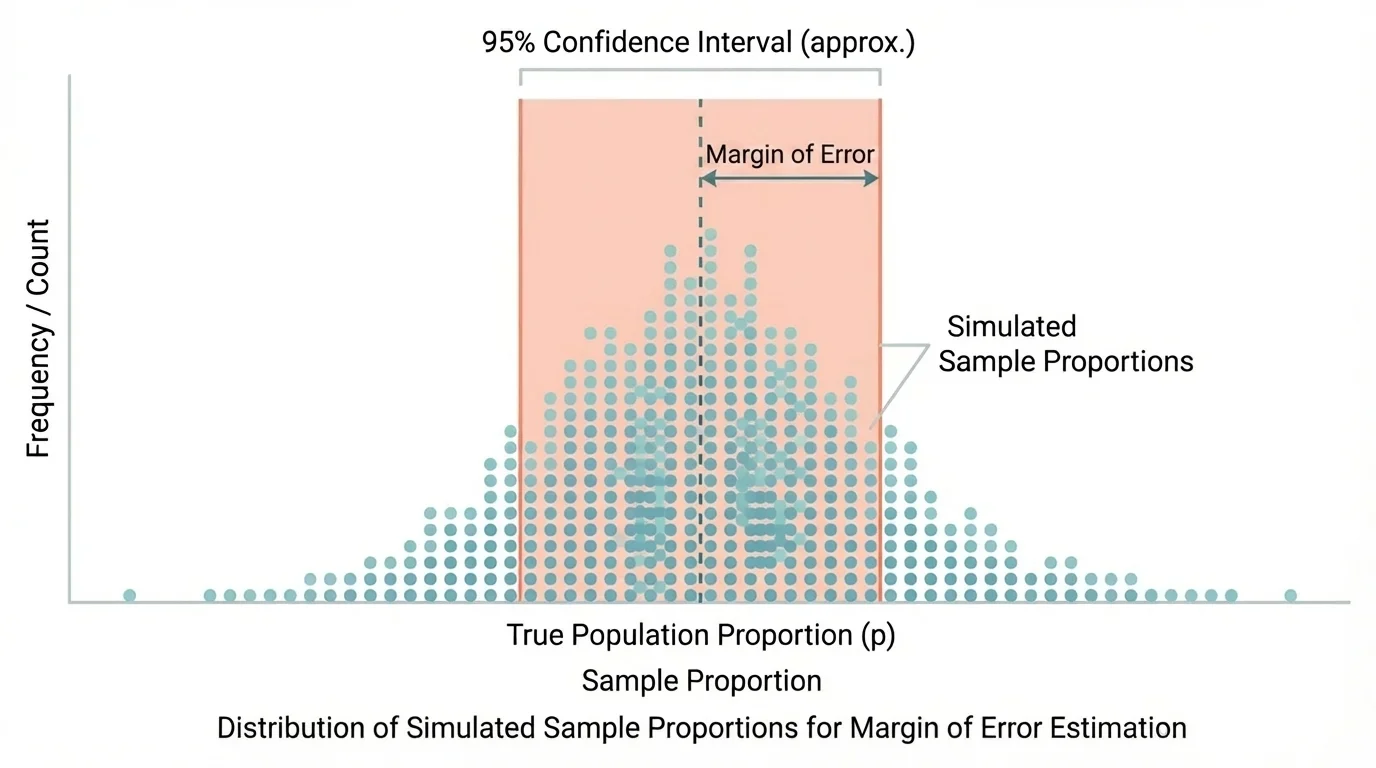
If most simulated sample proportions fall within about \(0.05\) of the true population proportion, then a reasonable margin of error is about \(0.05\). If our actual survey gives \(\hat{p} = 0.70\), we might estimate the population proportion as \(0.70 \pm 0.05\), or from \(0.65\) to \(0.75\).
For a mean, the same idea applies. Repeated random samples of the same size produce different sample means. A simulation lets us see how far those means typically fall from the population mean. That typical distance becomes the basis for a margin of error.
Large sample sizes reduce margin of error, but not in a simple doubling pattern. To cut the margin of error roughly in half, you usually need about four times as many observations.
This is one of the most surprising features of sampling: making a sample somewhat larger helps, but making it dramatically more precise requires much more data.
An estimate written as statistic \(\pm\) margin of error is often called an interval estimate. For example, if a sample mean of nightly sleep is \(6.8\) hours with a margin of error of \(0.3\) hours, then the interval estimate is from \(6.5\) to \(7.1\) hours.
The correct interpretation is careful: based on the sample and the sampling method, the population parameter is likely to be within that interval. It does not mean every individual value lies in that interval. A sleep estimate from \(6.5\) to \(7.1\) hours does not mean every student sleeps in that range; it refers to the population mean.
Likewise, if a survey estimates that \(52\%\) of students support a later start time with a margin of error of \(4\%\), then the estimated population proportion is between \(48\%\) and \(56\%\). Because \(50\%\) lies in that interval, the data do not strongly rule out an evenly split student body.
The ideas become clearer when we calculate and interpret actual estimates.
Worked example 1: Estimating a population proportion
A random sample of \(200\) students is asked whether they participate in at least one school club. In the sample, \(126\) say yes. Estimate the population proportion.
Step 1: Identify the sample proportion formula.
\[\hat{p} = \frac{\textrm{number with the characteristic}}{n}\]
Step 2: Substitute the sample values.
\(\hat{p} = \dfrac{126}{200} = 0.63\)
Step 3: Interpret the result.
The point estimate for the population proportion is \(0.63\), or \(63\%\).
A reasonable conclusion is that about 63% of all students at the school may participate in at least one club, assuming the sample is random and representative.
Notice that we are not claiming exactly \(63\%\). We are using sample evidence to estimate a population value.
Worked example 2: Estimating a population mean
A random sample of \(5\) students reports the number of hours they studied last week: \(4, 6, 5, 3, 7\). Estimate the population mean study time.
Step 1: Add the sample values.
\(4 + 6 + 5 + 3 + 7 = 25\)
Step 2: Divide by the sample size.
\(\bar{x} = \dfrac{25}{5} = 5\)
Step 3: Interpret the result.
The sample mean is \(5\) hours.
The point estimate for the population mean study time is 5 hours.
With such a small sample, the estimate may vary a lot from one sample to another. That is why margin of error and sample size matter.
Worked example 3: Developing a margin of error from simulation
A random sample of \(100\) students finds that \(58\) prefer digital textbooks to printed textbooks, so \(\hat{p} = 0.58\). A simulation takes \(1{,}000\) random samples of size \(100\) from a model based on this result. About \(95\%\) of the simulated sample proportions fall within \(0.10\) of \(0.58\).
Step 1: Use the simulated spread to estimate the margin of error.
The margin of error is about \(0.10\).
Step 2: Build the interval estimate.
\(0.58 - 0.10 = 0.48\) and \(0.58 + 0.10 = 0.68\)
Step 3: State the interval.
\[0.48 \leq p \leq 0.68\]
The estimated population proportion is from 48% to 68%.
The simulation does not prove the true value. It shows what kinds of sample-to-sample differences are typical under random sampling, which is exactly what margin of error is meant to capture.
Worked example 4: Estimating a population mean with a simulated margin of error
A sample survey of \(80\) students gives a mean commute time of \(18\) minutes. A simulation of repeated random samples of size \(80\) shows that sample means are usually within \(2\) minutes of the population mean.
Step 1: Identify the point estimate and margin of error.
Point estimate: \(18\) minutes. Margin of error: \(2\) minutes.
Step 2: Form the interval.
\(18 - 2 = 16\) and \(18 + 2 = 20\)
Step 3: Interpret the interval.
The estimated population mean commute time is between \(16\) and \(20\) minutes.
This interval describes the likely location of the population mean, not the commute time of every individual student.
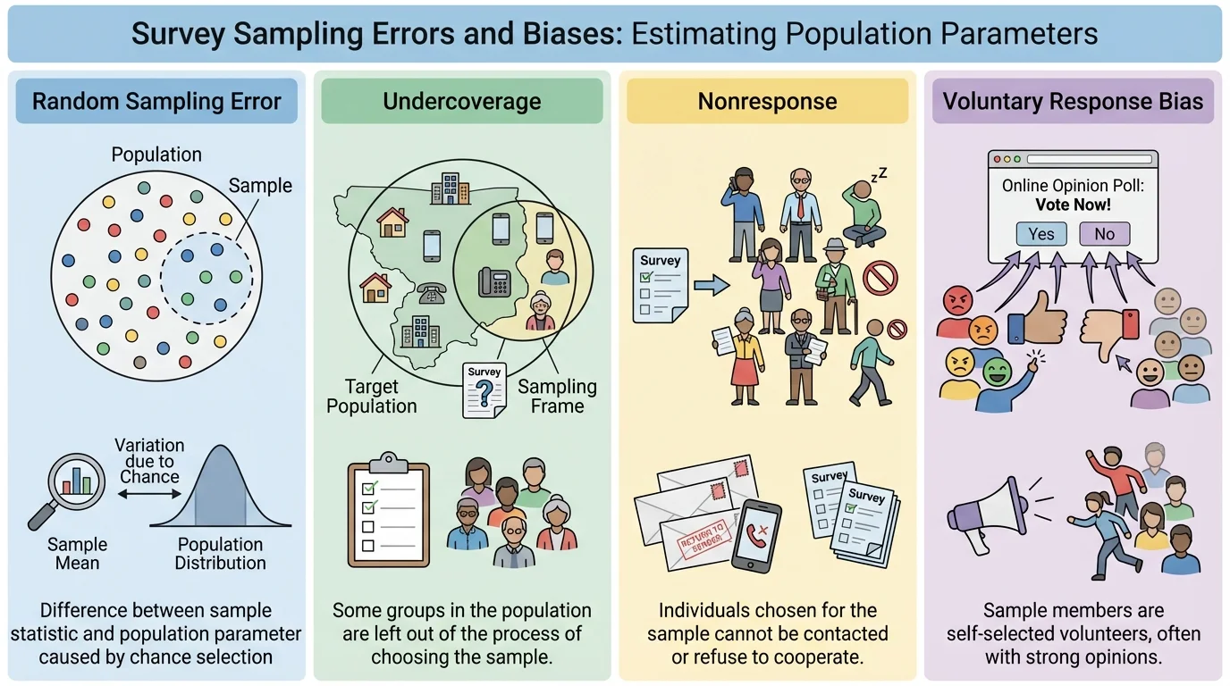
Margin of error is useful, but it does not cover every possible problem. Random sampling variation is only one source of uncertainty. A survey can still be misleading if the method itself is flawed.
Undercoverage happens when some groups in the population are less likely to be included. Nonresponse happens when selected individuals do not respond. Response bias can happen if people do not answer honestly or if question wording influences responses. A voluntary response sample, such as an open online poll, often overrepresents people with strong opinions.
For example, a survey asking, "Don't you agree the cafeteria prices are too high?" is leading. The wording pushes respondents toward a certain answer. No margin of error can fix that kind of bias.
Similarly, if only students who are active on a school social media page answer a poll about homework stress, the results may not represent all students. This is why a good inference always depends on both the numbers and the method used to gather them.
| Issue | What it means | Effect on conclusions |
|---|---|---|
| Random sampling variation | Different random samples give different results | Creates uncertainty measured by margin of error |
| Undercoverage | Some groups are left out | Can bias estimates |
| Nonresponse | Chosen people do not answer | Can bias estimates if nonresponders differ from responders |
| Response bias | Answers are influenced by wording or dishonesty | Can distort results |
| Voluntary response | People choose themselves to participate | Often overrepresents strong opinions |
Table 1. Common sources of uncertainty and bias in sample surveys.
Later, when comparing two surveys, it is not enough to compare only their margins of error. We also have to ask whether each survey used a sound sampling method, just as we saw with the method problems summarized in [Figure 3].
Sample surveys and margins of error appear everywhere. Election polling estimates voter support. Public health surveys estimate vaccination rates or average sleep time. Environmental scientists sample water from a limited number of sites to estimate average pollution levels in a larger area. Businesses survey customers to estimate satisfaction or the proportion likely to recommend a product.
In sports analytics, a team might sample player performance data to estimate an average training improvement. In education, districts may survey a random sample of families to estimate the proportion who support schedule changes. These are not just school exercises; they are the tools used to make real decisions.
"The goal of statistics is not certainty, but informed judgment under uncertainty."
That idea is especially important in public discussions. A survey should not be treated like a perfect snapshot of reality. It is evidence, and good evidence includes both an estimate and an honest measure of uncertainty.
When you read or conduct a survey, ask several questions. Was the sample random? Was the sample large enough? What population is the survey trying to describe? Is the estimate a mean or a proportion? What is the margin of error? Are there possible sources of bias?
A strong conclusion sounds like this: "Based on a random sample of \(300\) students, about \(54\%\) support the new schedule, with a margin of error of about \(5\%\)." A weak conclusion sounds like this: "Most students definitely support the new schedule." The first statement respects uncertainty. The second goes beyond what the data justify.
The big idea is not just calculating \(\bar{x}\) or \(\hat{p}\). It is learning how evidence from a sample can support a claim about a population while still recognizing limits. That balance between evidence and caution is the heart of statistical inference.