A weather app might say there is a chance of rain tomorrow, but what if you want the chance of rain and wind, or the chance that your team wins and scores more than one goal? Real situations often involve more than one event happening together. Probability helps us answer these questions fairly and logically by looking at all possible outcomes and finding how many match the event we care about.
When there is more than one step in a chance process, we call the result a compound event. The big idea is actually the same as with a simple event: probability is still a comparison between the number of favorable outcomes and the total number of outcomes in the sample space. The only difference is that the sample space may be larger and may need an organized method to make sure nothing is missed.
Many games, experiments, and real-life decisions depend on compound events. A compound event can include phrases like "and," "or," "both," or "at least one." For example, tossing two coins, spinning two spinners, choosing an outfit, or checking whether a student chosen at random is in band and plays soccer are all compound situations. If you can describe all possible outcomes clearly, then you can find the probability.
Compound events matter because our intuition is not always reliable. People often guess probabilities based on what feels likely, but organized counting gives a correct answer. That is one reason probability is used in science, sports, medicine, and manufacturing.
You already know that for a simple event, probability can be written as
\[P(\textrm{event}) = \frac{\textrm{number of favorable outcomes}}{\textrm{total number of outcomes}}\]
The same idea works for compound events. The challenge is building the full sample space correctly.
A compound event is an event made from two or more simple events. For example, "rolling an even number and flipping heads" combines two separate actions. A outcome is one possible result, such as \((H,4)\) for getting heads on a coin and a \(4\) on a number cube.
The probability of a compound event is the fraction of outcomes in the sample space for which the compound event occurs. That sentence is the heart of this topic. If the sample space has \(12\) equally likely outcomes and the event happens in \(3\) of them, then the probability is \(\dfrac{3}{12} = \dfrac{1}{4}\).
Sample space is the set of all possible outcomes of a chance experiment.
Compound event is an event that combines two or more simple events.
Favorable outcomes are the outcomes in the sample space that satisfy the event.
When outcomes are equally likely, each outcome has the same chance of happening. In grade \(7\), many probability problems assume equally likely outcomes, such as fair coins, fair number cubes, and fair spinners divided into equal sections. In these cases, counting outcomes works well.
Suppose you flip a coin and roll a number cube. The possible outcomes are \((H,1), (H,2), (H,3), (H,4), (H,5), (H,6), (T,1), (T,2), (T,3), (T,4), (T,5), (T,6)\). There are \(12\) outcomes total. If the event is "tails and an even number," the favorable outcomes are \((T,2), (T,4), (T,6)\), so the probability is \(\dfrac{3}{12} = \dfrac{1}{4}\).
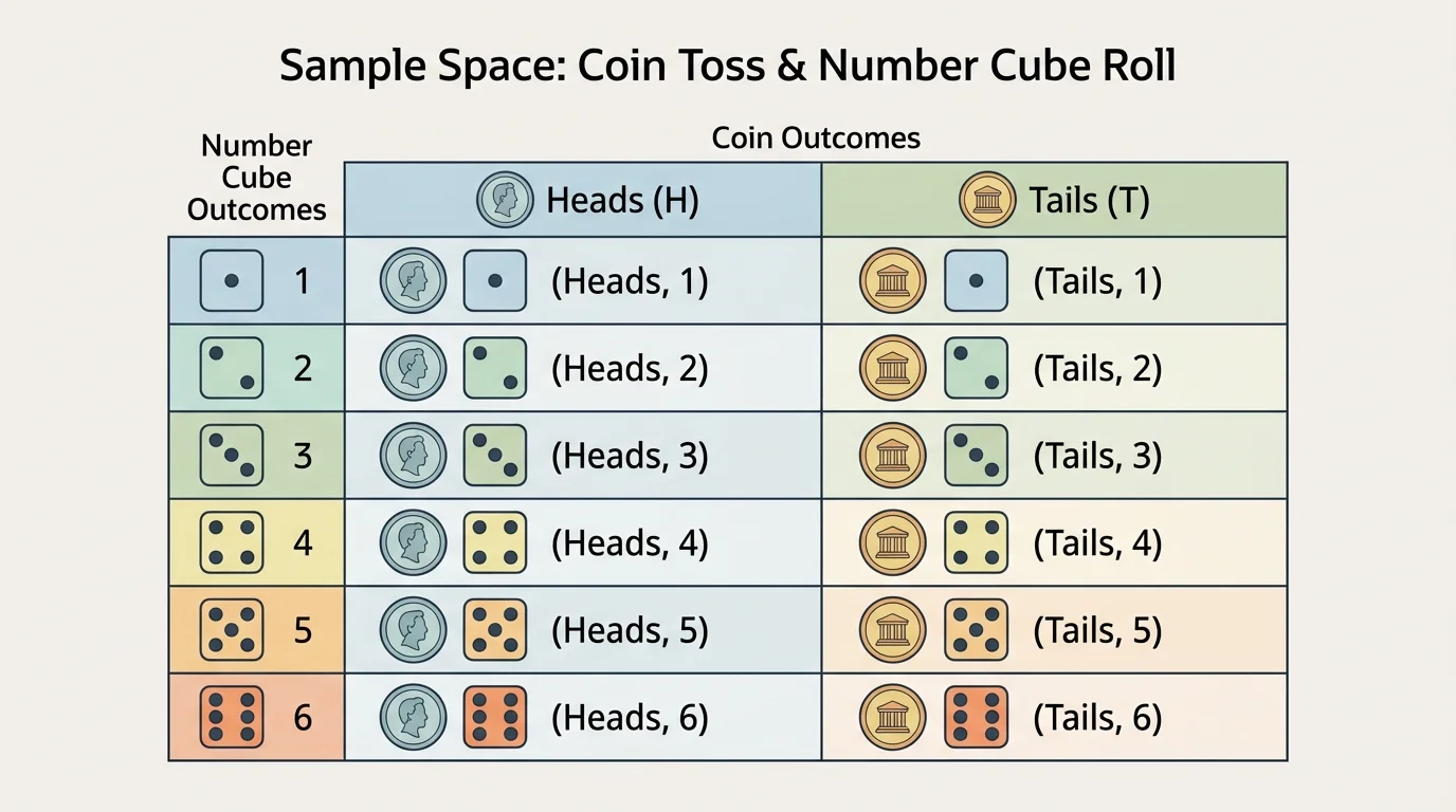
One useful way to build a sample space is an organized list. This means listing all outcomes carefully in a pattern so that none are skipped and none are repeated. As [Figure 1] shows, another helpful method is a table, which keeps the sample space complete and easy to read for a coin-and-number-cube experiment.
If you toss a coin and roll a number cube, a table can display coin results across the top and numbers down the side. Each box then shows one outcome pair. This is especially helpful because it makes it clear that \(2 \times 6 = 12\) total outcomes exist. Every pair must be counted once.
Tables are also useful when comparing two spinners, two number cubes, or two choices from different categories. For example, if one spinner has colors red, blue, and green and another has numbers \(1, 2, 3, 4\), then there are \(3 \times 4 = 12\) possible ordered outcomes.
Sometimes an organized list is more natural than a table. If you roll two number cubes, you can list outcomes in order: \((1,1), (1,2), (1,3), ..., (6,6)\). The order matters because \((2,5)\) and \((5,2)\) are different outcomes when two separate number cubes are rolled.
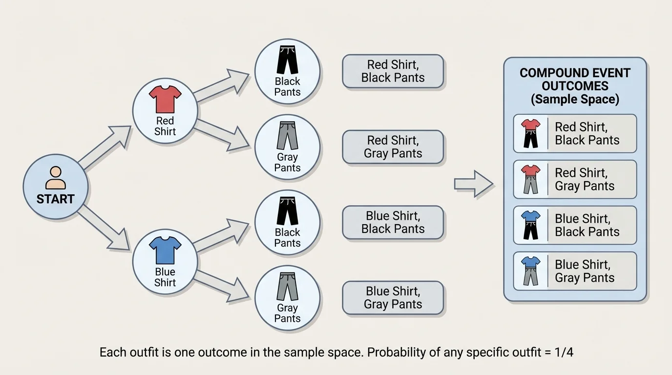
As [Figure 2] illustrates, a tree diagram is another way to organize a compound event. It uses branches to show each possible choice at each stage, and each complete path represents one outcome. This branching structure organizes multi-step events clearly.
Suppose a student chooses one shirt from red or blue, then one pair of pants from black or gray. Start with two branches for shirts. From each shirt branch, draw two more branches for pants. The completed paths are red-black, red-gray, blue-black, and blue-gray. There are \(4\) outcomes.
Tree diagrams are especially helpful when there are several steps in order, such as flipping a coin twice or selecting from one category and then another. They show not only the total number of outcomes but also how each outcome is formed.
Later, when you check whether you missed any outcomes, the complete paths in the tree act like a checklist. That is why tree diagrams are one of the best tools for compound probability.
How to find probability from a sample space
First, build the full sample space using an organized list, table, or tree diagram. Next, identify which outcomes make the event true. Finally, write probability as the fraction of favorable outcomes over total outcomes. If possible, simplify the fraction.
Once the sample space is complete, the calculation is straightforward:
\[P(\textrm{compound event}) = \frac{\textrm{number of outcomes where the event occurs}}{\textrm{total number of outcomes in the sample space}}\]
For example, if two coins are tossed, the sample space is \(\{HH, HT, TH, TT\}\). Consider the event "exactly one head." The favorable outcomes are \(HT\) and \(TH\), so
\[P(\textrm{exactly one head}) = \frac{2}{4} = \frac{1}{2}\]
Notice that the event is not "a head appears somewhere in the outcome" in a vague way. You must count the exact outcomes that fit the words of the event. Precision matters in probability.
The best way to understand compound probability is to see complete solutions from start to finish.
Worked example 1
A fair coin is flipped and a fair number cube is rolled. What is the probability of getting heads and a number greater than \(4\)?
Step 1: List the sample space size.
The coin has \(2\) outcomes and the number cube has \(6\) outcomes, so there are \(2 \times 6 = 12\) outcomes total.
Step 2: Find the favorable outcomes.
Numbers greater than \(4\) are \(5\) and \(6\). With heads, the favorable outcomes are \((H,5)\) and \((H,6)\).
Step 3: Write the probability.
\[P(\textrm{heads and number greater than }4) = \frac{2}{12} = \frac{1}{6}\]
The probability is \(\dfrac{1}{6}\).
Notice how the full sample space makes the answer trustworthy. Without listing or organizing, it is easy to overlook an outcome.
Worked example 2
Two fair coins are tossed. What is the probability of getting at least one tail?
Step 1: Write the sample space.
The outcomes are \(HH, HT, TH, TT\).
Step 2: Identify favorable outcomes.
At least one tail means one or more tails, so the favorable outcomes are \(HT, TH, TT\).
Step 3: Write the fraction.
\[P(\textrm{at least one tail}) = \frac{3}{4}\]
The probability is \(\dfrac{3}{4}\).
The phrase "at least one" often causes confusion. It includes outcomes with exactly one and with more than one.
Worked example 3
A spinner has four equal sections labeled \(1, 2, 3, 4\). It is spun twice. What is the probability that the sum is \(5\)?
Step 1: Count total outcomes.
Each spin has \(4\) outcomes, so the total is \(4 \times 4 = 16\).
Step 2: List outcomes with sum \(5\).
The favorable outcomes are \((1,4), (2,3), (3,2), (4,1)\).
Step 3: Write and simplify.
\[P(\textrm{sum }5) = \frac{4}{16} = \frac{1}{4}\]
The probability is \(\dfrac{1}{4}\).
Here order matters in the sample space because the first spin and second spin are separate stages. That is why \((1,4)\) and \((4,1)\) are counted separately.
Worked example 4
A bag contains cards labeled \(A, B, C\). One card is chosen, replaced, and then another card is chosen. What is the probability of choosing \(A\) both times?
Step 1: Count total outcomes.
There are \(3\) choices for the first draw and \(3\) for the second, so there are \(3 \times 3 = 9\) outcomes.
Step 2: Find favorable outcomes.
Only one outcome works: \((A,A)\).
Step 3: Compute the probability.
\[P(\textrm{A both times}) = \frac{1}{9}\]
The probability is \(\dfrac{1}{9}\).
Replacement means the first choice does not change the second sample space. That is why the second draw still has all \(3\) possible labels available.
Different tools can lead to the same answer. A table, organized list, or tree diagram all represent the same sample space in different ways. For the outfit example, the tree diagram in [Figure 2] makes the order of choices especially clear. For the coin-and-number-cube example, a table like [Figure 1] is often faster to scan.
The important thing is not which method looks most sophisticated. The important thing is whether the method includes every possible outcome exactly once.
| Method | Best use | Strength |
|---|---|---|
| Organized list | Small sample spaces | Simple and direct |
| Table | Two sets of outcomes | Easy to count pairs |
| Tree diagram | Multi-step events in order | Shows branching paths clearly |
| Simulation | Large or complex experiments | Estimates probability from repeated trials |
Table 1. Comparison of common methods for finding probabilities of compound events.
Sometimes building the full sample space is possible but time-consuming, and sometimes a simulation is useful for checking results. A simulation is an experiment that models a real chance process. Repeating it many times gives an experimental probability, which is based on actual trial results rather than perfect counting.
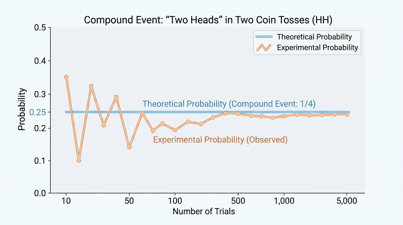
For example, you could simulate flipping two coins by using a random number generator, or simulate drawing colored objects by using slips of paper in a cup. Over many trials, the experimental probability usually gets closer to the theoretical probability, as [Figure 3] shows.
If the theoretical probability of an event is \(\dfrac{1}{4}\), then after a small number of trials the experimental result might be \(\dfrac{3}{10}\) or \(\dfrac{2}{9}\). But after many more trials, the relative frequency often settles closer to \(\dfrac{1}{4}\). This is one reason probability is connected to long-run patterns, not just one short experiment.
Simulation does not replace theoretical probability when the sample space is easy to find. Instead, it supports understanding. It also becomes very helpful when an event has many stages or when technology can run thousands of trials quickly.
Computer scientists and engineers use simulations constantly. They test traffic patterns, weather models, and even space missions by running many repeated trials before decisions are made in the real world.
Compound probability appears in many real situations. In sports, a coach may study the chance that a player makes the first free throw and the second free throw. In manufacturing, a company may track the probability that a product passes two separate quality checks. In medicine, researchers may examine the chance that a treatment helps a patient and causes no serious side effects.
Weather forecasts also involve compound thinking. The chance of "rain and strong wind" is different from the chance of "rain or strong wind." In games, knowing the probability of rolling a certain sum on two number cubes helps players make better decisions. Behind each of these situations is the same idea: count the outcomes in the sample space where the event occurs.
Even choosing passwords or predicting combinations in technology relies on counting outcomes. The logic of compound events helps people evaluate risk, design fair games, and understand data.
One common mistake is leaving outcomes out of the sample space. If the sample space is incomplete, the probability will be wrong. Another mistake is counting the same outcome more than once. Organized methods prevent both errors.
A second mistake is misunderstanding event language. "Exactly one," "at least one," and "both" mean different things. For example, with two coin tosses, "exactly one head" is \(HT\) or \(TH\), but "at least one head" is \(HH, HT, TH\).
A third mistake is forgetting whether order matters. For two separate spins or rolls, order usually matters because the first result and second result are recorded separately. That is why outcomes like \((2,3)\) and \((3,2)\) may both belong in the sample space.
The graph of simulation results in [Figure 3] also reminds us not to expect short experiments to match theoretical probability perfectly. Small samples can bounce around a lot, but larger samples tend to be steadier.
The main rule does not change from simple events to compound events. You still compare favorable outcomes with total outcomes. What changes is the size and structure of the sample space.
Whenever you face a compound event, ask yourself three questions: What are all possible outcomes? Which of those outcomes make the event true? What fraction do they form? If you can answer those questions carefully, you can solve the probability problem.