A video game character turns, stretches, and flips across a screen because of matrix multiplication. The same mathematics helps animate movies, guide robots, and process data. What looks like motion or change is often a matrix taking one vector and producing another. This idea is powerful because it turns geometry into computation: a matrix can act like a machine, and a vector is the object that goes into it.
A vector is often used to represent a quantity with both size and direction, or simply an ordered list of numbers. In matrix work, we usually write a vector as a column matrix. For example, the vector with components \(3\) and \(-1\) can be written as
\[\begin{bmatrix}3\\-1\end{bmatrix}\]
This is a \(2 \times 1\) matrix because it has \(2\) rows and \(1\) column. Likewise,
\[\begin{bmatrix}4\\0\\7\end{bmatrix}\]
is a \(3 \times 1\) vector.
You already know that matrix dimensions are written as rows by columns. A matrix with \(2\) rows and \(3\) columns is a \(2 \times 3\) matrix. This dimension language is essential because multiplication depends on matching dimensions correctly.
When we use vectors in this form, each entry can represent something meaningful: position, velocity, change in profit, force, or coordinates in the plane. A vector is not just a list of numbers. It is often an input to a rule that transforms it.
Suppose we have a matrix \(A\) and a vector \(\mathbf{v}\). If \(A\) has dimensions \(m \times n\), then \(\mathbf{v}\) must have dimensions \(n \times 1\) for the product \(A\mathbf{v}\) to be defined. The result will then have dimensions \(m \times 1\).
In symbols,
\[(m \times n)(n \times 1) = (m \times 1)\]
The inside numbers must match. That matching value \(n\) tells us that each row of the matrix has exactly as many entries as the vector has entries.
Dimension tells the size of a matrix in rows and columns. Compatible dimensions means the number of columns in the first matrix equals the number of rows in the second. A column matrix is a matrix with one column, often used to represent a vector.
For example, a \(3 \times 2\) matrix can multiply a \(2 \times 1\) vector and give a \(3 \times 1\) vector. But a \(3 \times 2\) matrix cannot multiply a \(3 \times 1\) vector, because \(2 \neq 3\).
This is one of the first places students make mistakes. The matrix does not multiply just any vector. The number of columns in the matrix controls what length of input vector is allowed.
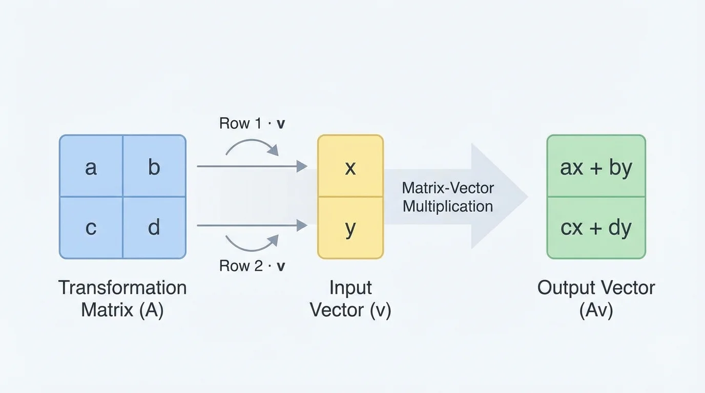
Matrix-vector multiplication works by taking each row of the matrix and combining it with the vector through a dot product. Each row creates one entry in the output vector, so the result has as many entries as the matrix has rows.
If
\[A = \begin{bmatrix}a & b \\ c & d\end{bmatrix}, \quad \mathbf{v} = \begin{bmatrix}x \\ y\end{bmatrix}\]
then
\[A\mathbf{v} = \begin{bmatrix}ax + by \\ cx + dy\end{bmatrix}\]
The top entry comes from the first row of \(A\): \(a\) and \(b\) interact with \(x\) and \(y\). The bottom entry comes from the second row.
You can think of this as the matrix reading the input vector and producing a new vector according to its row rules. If the matrix has \(3\) rows, the output will have \(3\) entries. If the matrix has \(2\) rows, the output will have \(2\) entries.
Worked example 1
Multiply \(\begin{bmatrix}2 & 1 \\ -3 & 4\end{bmatrix}\) by \(\begin{bmatrix}5 \\ -2\end{bmatrix}\).
Step 1: Check dimensions.
The matrix is \(2 \times 2\) and the vector is \(2 \times 1\), so multiplication is defined. The result will be a \(2 \times 1\) vector.
Step 2: Compute the first entry.
Use the first row: \((2)(5) + (1)(-2) = 10 - 2 = 8\).
Step 3: Compute the second entry.
Use the second row: \((-3)(5) + (4)(-2) = -15 - 8 = -23\).
Step 4: Write the result as a vector.
\[\begin{bmatrix}2 & 1 \\ -3 & 4\end{bmatrix}\begin{bmatrix}5 \\ -2\end{bmatrix} = \begin{bmatrix}8 \\ -23\end{bmatrix}\]
The new vector is \(\begin{bmatrix}8 \\ -23\end{bmatrix}\).
Notice how the computation in this example follows the structure shown earlier in [Figure 1]. Each output entry comes from one row of the matrix acting on the entire input vector, not from multiplying entries straight down.
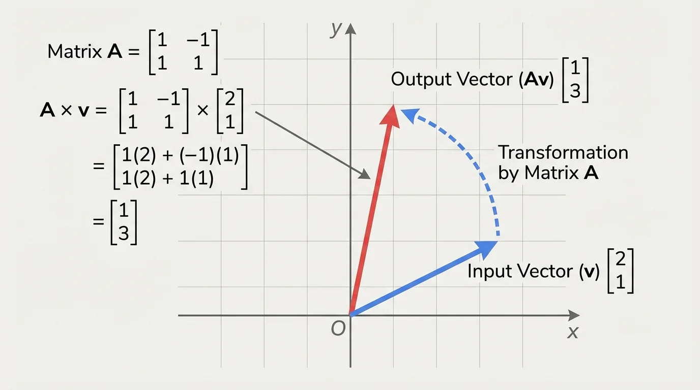
A transformation is a rule that takes an input and produces an output. In matrix language, a matrix transforms a vector into another vector. In two dimensions, this often means a point or arrow in the coordinate plane moves to a new position.
[Figure 2] If a vector \(\mathbf{v}\) represents a point or direction in the plane, then multiplying by a matrix \(A\) gives a new vector \(A\mathbf{v}\). The matrix controls how all vectors are changed. Some matrices stretch vectors, some reflect them, some rotate them, and some shear them.
For instance, if
\[A = \begin{bmatrix}2 & 0 \\ 0 & 2\end{bmatrix}\]
then every vector is doubled in length:
\[A\begin{bmatrix}x \\ y\end{bmatrix} = \begin{bmatrix}2x \\ 2y\end{bmatrix}\]
That matrix scales the plane away from the origin by a factor of \(2\).
Why the origin stays fixed
For any matrix \(A\), the zero vector stays the zero vector because \(A\begin{bmatrix}0\\0\end{bmatrix} = \begin{bmatrix}0\\0\end{bmatrix}\). This is one reason matrix transformations are called linear transformations: they preserve the origin and change vectors in a consistent algebraic way.
Geometrically, this is a big idea. The matrix is not changing just one vector. It defines a rule for every vector of the correct size. Once you know the matrix, you know how the entire space is transformed.
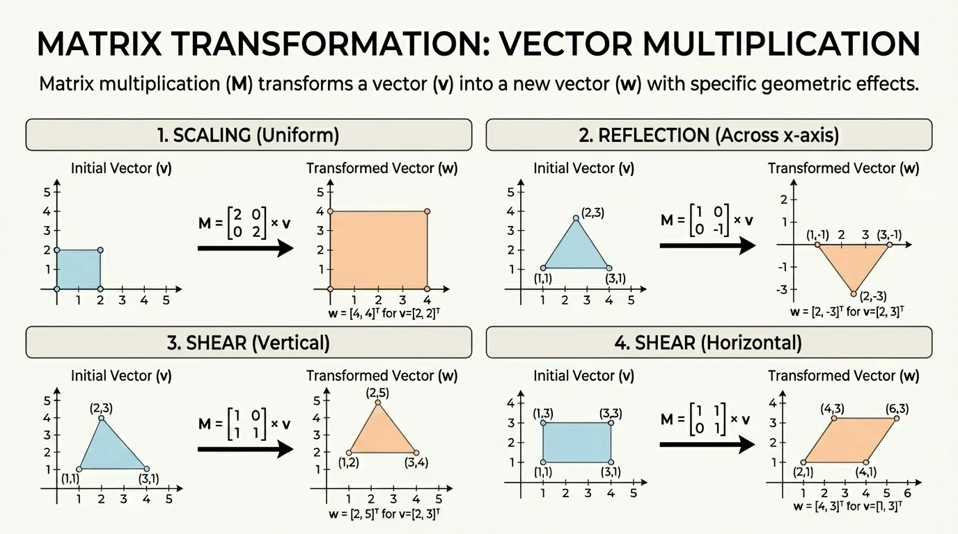
Different matrices create different geometric effects, and [Figure 3] compares several of the most important ones. Even simple matrices can create dramatic changes in the plane.
Scaling: A scaling matrix changes size. For example,
\[\begin{bmatrix}3 & 0 \\ 0 & 1\end{bmatrix}\begin{bmatrix}x \\ y\end{bmatrix} = \begin{bmatrix}3x \\ y\end{bmatrix}\]
This stretches horizontally by a factor of \(3\) while leaving the vertical coordinate unchanged.
Reflection across the \(x\)-axis:
\[\begin{bmatrix}1 & 0 \\ 0 & -1\end{bmatrix}\begin{bmatrix}x \\ y\end{bmatrix} = \begin{bmatrix}x \\ -y\end{bmatrix}\]
This keeps the \(x\)-coordinate the same but flips the \(y\)-coordinate.
Shear:
\[\begin{bmatrix}1 & 2 \\ 0 & 1\end{bmatrix}\begin{bmatrix}x \\ y\end{bmatrix} = \begin{bmatrix}x + 2y \\ y\end{bmatrix}\]
A shear slants the plane. Points move sideways depending on their height.
Rotation by \(90^\circ\) counterclockwise:
\[\begin{bmatrix}0 & -1 \\ 1 & 0\end{bmatrix}\begin{bmatrix}x \\ y\end{bmatrix} = \begin{bmatrix}-y \\ x\end{bmatrix}\]
This turns every vector by \(90^\circ\) around the origin. A point at \((1,0)\) goes to \((0,1)\), and a point at \((0,1)\) goes to \((-1,0)\).
Computer graphics often build complex motion from simple matrices like scaling, rotation, and reflection. A digital object on a screen can be moved thousands of times per second using repeated matrix operations.
Later, when you compare outputs, [Figure 3] helps explain why some matrices preserve shape better than others. A reflection keeps lengths the same, while a scaling matrix changes them, and a shear changes angles even if some lengths look similar.
Careful examples are the best way to make these ideas feel natural. Watch how dimensions, arithmetic, and interpretation all work together.
Worked example 2
Determine whether the product \(\begin{bmatrix}1 & 4 & -2 \\ 0 & 3 & 5\end{bmatrix}\begin{bmatrix}7 \\ -1 \\ 2\end{bmatrix}\) is defined, and if so, compute it.
Step 1: Check dimensions.
The matrix is \(2 \times 3\) and the vector is \(3 \times 1\). Since the inner dimensions match, the product is defined and the result will be \(2 \times 1\).
Step 2: Compute the first entry.
\((1)(7) + (4)(-1) + (-2)(2) = 7 - 4 - 4 = -1\).
Step 3: Compute the second entry.
\((0)(7) + (3)(-1) + (5)(2) = 0 - 3 + 10 = 7\).
Step 4: State the product.
\[\begin{bmatrix}1 & 4 & -2 \\ 0 & 3 & 5\end{bmatrix}\begin{bmatrix}7 \\ -1 \\ 2\end{bmatrix} = \begin{bmatrix}-1 \\ 7\end{bmatrix}\]
The product is defined, and the output vector is \(\begin{bmatrix}-1 \\ 7\end{bmatrix}\).
That example shows that the matrix does not need to be square. A non-square matrix can still act on a vector, as long as the dimensions are compatible.
Worked example 3
Use the matrix \(\begin{bmatrix}1 & 0 \\ 0 & -1\end{bmatrix}\) to transform the vector \(\begin{bmatrix}3 \\ 5\end{bmatrix}\), and interpret the result geometrically.
Step 1: Multiply the matrix by the vector.
\[\begin{bmatrix}1 & 0 \\ 0 & -1\end{bmatrix}\begin{bmatrix}3 \\ 5\end{bmatrix} = \begin{bmatrix}(1)(3) + (0)(5) \\ (0)(3) + (-1)(5)\end{bmatrix} = \begin{bmatrix}3 \\ -5\end{bmatrix}\]
Step 2: Interpret the coordinates.
The \(x\)-coordinate stays \(3\), while the \(y\)-coordinate changes from \(5\) to \(-5\).
Step 3: Describe the transformation.
This is a reflection across the \(x\)-axis.
The vector \(\begin{bmatrix}3 \\ 5\end{bmatrix}\) is sent to \(\begin{bmatrix}3 \\ -5\end{bmatrix}\).
Geometric interpretation matters because matrix multiplication is more than arithmetic. It tells you what kind of change the matrix applies to space.
Worked example 4
Let \(A = \begin{bmatrix}2 & 0 \\ 0 & 2\end{bmatrix}\) and \(\mathbf{v} = \begin{bmatrix}-1 \\ 4\end{bmatrix}\). Find \(A\mathbf{v}\) and describe the transformation.
Step 1: Multiply.
\[A\mathbf{v} = \begin{bmatrix}2 & 0 \\ 0 & 2\end{bmatrix}\begin{bmatrix}-1 \\ 4\end{bmatrix} = \begin{bmatrix}-2 \\ 8\end{bmatrix}\]
Step 2: Compare input and output.
Each coordinate doubles: \(-1\) becomes \(-2\), and \(4\) becomes \(8\).
Step 3: Interpret the effect.
The matrix scales every vector by a factor of \(2\) from the origin.
The output vector points in the same direction as the original but has twice the length.
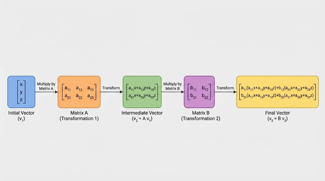
Sometimes one transformation is followed by another. Doing two transformations in sequence is called composition, and it shows how an input vector passes through one matrix, then another, to produce the final output.
[Figure 4] If a vector \(\mathbf{v}\) is first transformed by \(B\), giving \(B\mathbf{v}\), and then that result is transformed by \(A\), the overall output is
\[A(B\mathbf{v}) = (AB)\mathbf{v}\]
This means the single matrix \(AB\) represents the combined effect. The order matters: usually \(AB \neq BA\).
This order issue is one of the most important ideas in matrix transformations. Rotating then reflecting can produce a different result from reflecting then rotating. Matrices encode actions, and actions often depend on sequence.
Worked example 5
First reflect across the \(x\)-axis, then scale by a factor of \(2\). Apply this combined transformation to \(\begin{bmatrix}1 \\ 3\end{bmatrix}\).
Step 1: Write the matrices.
Reflection across the \(x\)-axis: \(R = \begin{bmatrix}1 & 0 \\ 0 & -1\end{bmatrix}\).
Scaling by \(2\): \(S = \begin{bmatrix}2 & 0 \\ 0 & 2\end{bmatrix}\).
Step 2: Apply the reflection first.
\[R\begin{bmatrix}1 \\ 3\end{bmatrix} = \begin{bmatrix}1 \\ -3\end{bmatrix}\]
Step 3: Apply the scaling to the reflected vector.
\[S\begin{bmatrix}1 \\ -3\end{bmatrix} = \begin{bmatrix}2 \\ -6\end{bmatrix}\]
Step 4: Find the combined matrix.
\[SR = \begin{bmatrix}2 & 0 \\ 0 & 2\end{bmatrix}\begin{bmatrix}1 & 0 \\ 0 & -1\end{bmatrix} = \begin{bmatrix}2 & 0 \\ 0 & -2\end{bmatrix}\]
Step 5: Verify using the combined matrix.
\[\begin{bmatrix}2 & 0 \\ 0 & -2\end{bmatrix}\begin{bmatrix}1 \\ 3\end{bmatrix} = \begin{bmatrix}2 \\ -6\end{bmatrix}\]
The final vector is \(\begin{bmatrix}2 \\ -6\end{bmatrix}\), and the single matrix \(SR\) captures the full transformation.
When you revisit sequential transformations, [Figure 4] makes the logic clearer: the output of the first matrix becomes the input of the second. This is why matrix multiplication naturally describes composition.
Matrices as transformations are not just classroom objects. They are practical tools in many fields.
In computer graphics, the position of an object on a screen can be stored using vectors. A matrix can rotate the object, stretch it, or flip it. Video games and animation software repeatedly multiply coordinate vectors by transformation matrices to update images smoothly.
In robotics, the direction and position of a robotic arm can be modeled with vectors. Matrices describe how one movement changes the arm's orientation. A sequence of matrices can model several joints moving one after another.
In data science and economics, vectors can represent quantities such as production levels or resource amounts. A matrix can represent how one set of values is converted into another, such as inputs becoming outputs in a system.
In physics, matrices are used to change coordinate systems and describe transformations of velocity or force components. If a force vector is measured in one orientation, a matrix can rewrite it in another orientation.
Input-output thinking
One of the most useful ways to understand a matrix is as an input-output rule. The vector is the input, the matrix is the machine, and the new vector is the output. This viewpoint connects algebra, geometry, and applications in technology.
That input-output viewpoint is exactly why the graph in [Figure 2] is so valuable: it turns the symbols into motion. You can see one vector become another under the rule defined by the matrix.
A common mistake is multiplying entries in matching positions straight down the columns. That is not matrix-vector multiplication. You must use each row of the matrix with the entire vector.
Another mistake is ignoring dimensions. Before calculating, always check whether the number of columns in the matrix equals the number of rows in the vector. If not, the product is undefined.
Students also sometimes think every matrix transformation preserves length or angle. That is false. Some matrices stretch, compress, or shear. The matrix determines the geometric effect.
Finally, order matters. If two matrices are applied in different orders, the final vector may change. This is one reason matrix multiplication is so useful: it captures process as well as quantity.
| Matrix | Effect on \(\begin{bmatrix}x \\ y\end{bmatrix}\) | Geometric meaning |
|---|---|---|
| \(\begin{bmatrix}2 & 0 \\ 0 & 2\end{bmatrix}\) | \(\begin{bmatrix}2x \\ 2y\end{bmatrix}\) | Scale by \(2\) |
| \(\begin{bmatrix}1 & 0 \\ 0 & -1\end{bmatrix}\) | \(\begin{bmatrix}x \\ -y\end{bmatrix}\) | Reflect across the \(x\)-axis |
| \(\begin{bmatrix}0 & -1 \\ 1 & 0\end{bmatrix}\) | \(\begin{bmatrix}-y \\ x\end{bmatrix}\) | Rotate \(90^\circ\) counterclockwise |
| \(\begin{bmatrix}1 & 2 \\ 0 & 1\end{bmatrix}\) | \(\begin{bmatrix}x + 2y \\ y\end{bmatrix}\) | Horizontal shear |
Table 1. Common \(2 \times 2\) matrices and the transformations they apply to vectors in the plane.
Once you become comfortable with these patterns, you start to see matrices not as arrays of numbers but as compact descriptions of change. That is the central idea: multiplying a vector by a suitable matrix creates a new vector, and the matrix tells you exactly how the transformation happens.