A school survey can look simple on the surface, but it can answer surprisingly deep questions. If students are asked for both their grade level and their favorite subject, the results can reveal more than just popularity. They can show whether preferences change by grade, whether certain groups are more likely to choose one subject than another, and whether two events are related or behave independently. That is exactly what a two-way frequency table helps us see.
Many real data sets classify each object by two different categories at the same time. A student may be in tenth grade and prefer science. A patient may be vaccinated and test negative. A basketball shot may be taken from the corner and be made or missed. When one object belongs to one category from each of two lists, the data can be organized into a table.
In probability, this matters because a single table can describe counts and also act as a sample space for experimental data. Instead of listing every outcome one by one, we organize outcomes by category and use the counts to estimate how likely different events are.
From earlier probability work, recall that a probability is the ratio of favorable outcomes to total outcomes. In data-based probability, those outcomes are often counts from a survey or experiment, so a probability is estimated by dividing one frequency by another.
For this lesson, suppose a random sample of students from a school was asked two questions at once: what grade are you in, and which subject do you favor most among math, science, and English?
A two-way frequency table, as organized in [Figure 1], places one category along the rows and the other along the columns. Each interior cell gives the number of objects that fit both categories at once. For example, one cell might show how many tenth-grade students favor science.
Suppose the survey results are recorded like this.
| Grade | Math | Science | English | Total |
|---|---|---|---|---|
| Ninth | \(18\) | \(22\) | \(10\) | \(50\) |
| Tenth | \(16\) | \(28\) | \(16\) | \(60\) |
| Eleventh | \(20\) | \(18\) | \(12\) | \(50\) |
| Total | \(54\) | \(68\) | \(38\) | \(160\) |
Table 1. Favorite subject by grade level for a random sample of \(160\) students.
The interior numbers, such as \(28\) in the tenth-grade science cell, are called joint frequencies because they count students in both categories at the same time. The totals at the ends of rows and columns are called marginal totals. They tell how many students are in a row category or column category regardless of the other variable.
The grand total is \(160\). That is the total sample size. Every count in the table is part of this whole.
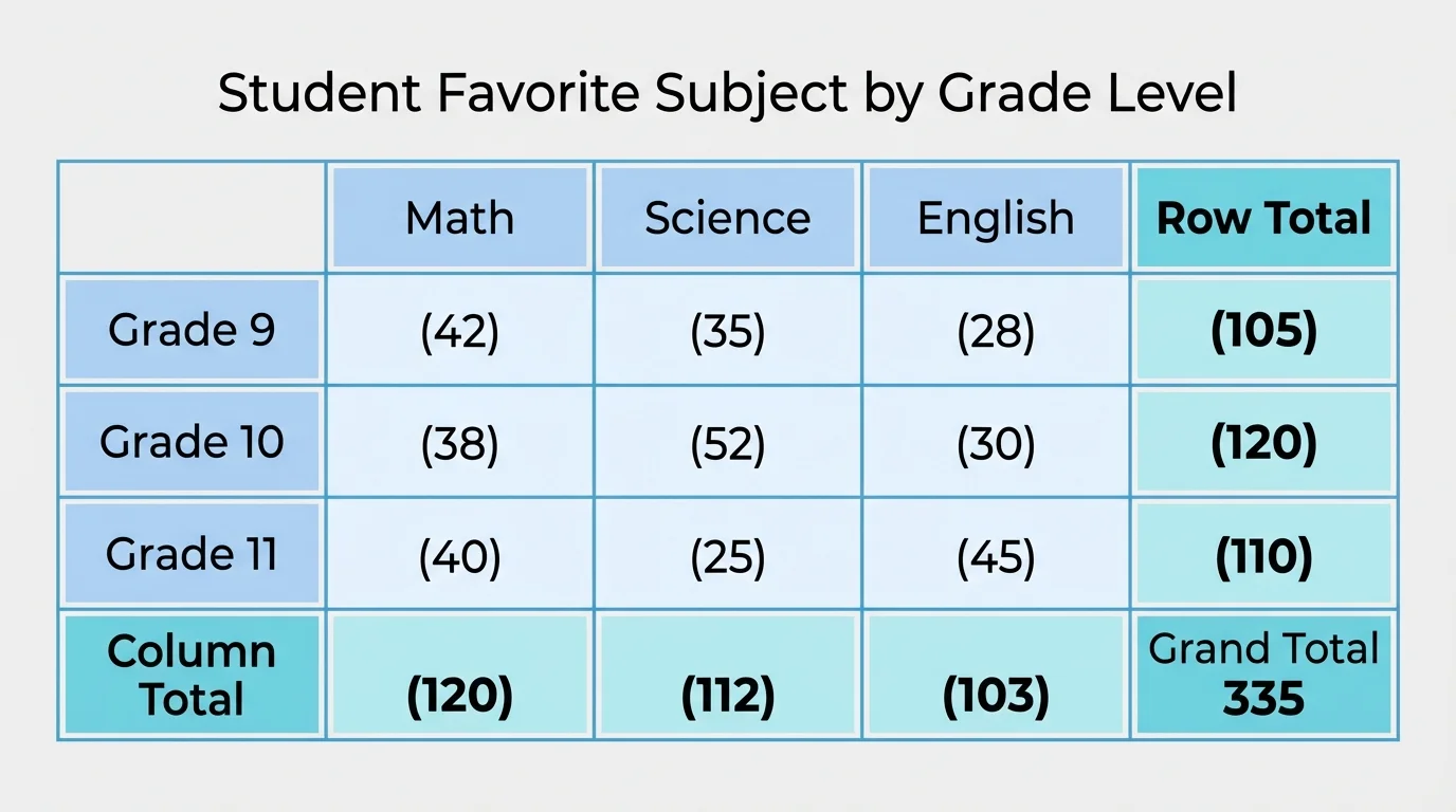
When constructing a table, you must make sure each person is counted exactly once in the correct cell. Since each student names only one favorite subject and belongs to one grade, the categories do not overlap within a row or within a column. That makes the totals meaningful and prevents double counting.
Joint frequency is the number in an interior cell of a two-way table, showing how many data values belong to both categories at once.
Marginal total is a row total or column total, showing how many data values belong to one category regardless of the other category.
Conditional probability is the probability of one event given that another event has already occurred.
Independent events are events for which knowing one happened does not change the probability of the other.
A useful check is that all row totals should add to the grand total, and all column totals should also add to the grand total. Here, \(50 + 60 + 50 = 160\), and also \(54 + 68 + 38 = 160\).
The table does more than store information. It can be treated as a sample space based on observed data. Every student in the sample belongs to one and only one cell, so the table represents all sampled outcomes.
For example, the event "the student favors science" corresponds to the entire science column. The event "the student is in tenth grade" corresponds to the entire tenth-grade row. The event "the student is in tenth grade and favors science" corresponds to the single cell where that row and column intersect.
How a two-way table becomes a probability model
If the sample is random, the table can be used to estimate probabilities for the larger population. A count divided by the grand total estimates an overall probability. A count divided by a row total or column total estimates a conditional probability, depending on which condition is given.
This is why two-way tables are so powerful: they connect statistics and probability. The data are collected as frequencies, but then those same counts are used to estimate probabilities and relationships.
A conditional probability changes the sample space. Instead of looking at all \(160\) students, we look only at the students who satisfy the given condition. The narrowing shown in [Figure 2] is the heart of the idea: "given tenth grade" means we ignore all rows except the tenth-grade row.
In symbols, the conditional probability of event \(A\) given event \(B\) is
\[P(A \mid B) = \frac{P(A \cap B)}{P(B)}\]
Using counts from a table, this becomes \(P(A \mid B) = \dfrac{\textrm{count in }A \cap B}{\textrm{count in }B}\). In words, divide the number in both events by the number in the given event.
To estimate the probability that a randomly selected student favors science given that the student is in tenth grade, we use only the tenth-grade row. There are \(60\) tenth graders, and \(28\) of them favor science. So
\[P(\textrm{Science} \mid \textrm{Tenth}) = \frac{28}{60} = \frac{7}{15} \approx 0.467\]
This means the estimated probability is about \(0.467\), or about \(46.7\%\).
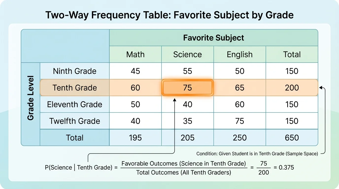
The denominator comes from the condition. If the phrase says "given tenth grade," the denominator is the total number of tenth-grade students. If the phrase said "given science," the denominator would instead be the total number of students who favor science.
This small wording difference matters a lot. Conditional probability always asks, "What group am I restricting attention to?"
Now do the same calculation for the other subjects among tenth graders. Since there are \(60\) tenth-grade students,
\[P(\textrm{Math} \mid \textrm{Tenth}) = \frac{16}{60} = \frac{4}{15} \approx 0.267\]
and
\[P(\textrm{English} \mid \textrm{Tenth}) = \frac{16}{60} = \frac{4}{15} \approx 0.267\]
Comparing these results shows that among tenth-grade students in this sample, science is favored more often than math or English. The probabilities are approximately \(46.7\%\), \(26.7\%\), and \(26.7\%\), respectively.
Notice something important: when the categories are complete choices within one row, the conditional probabilities across that row must add to \(1\). Here,
\[\frac{16}{60} + \frac{28}{60} + \frac{16}{60} = \frac{60}{60} = 1\]
That makes sense because every tenth-grade student must prefer one of the three listed subjects.
Conditional probabilities are used in medicine, marketing, and machine learning because decisions often depend on already knowing one piece of information. A test result, an age group, or a customer preference can completely change the relevant probability.
We can also compare science preference across grades:
\[P(\textrm{Science} \mid \textrm{Ninth}) = \frac{22}{50} = 0.44\]
\[P(\textrm{Science} \mid \textrm{Tenth}) = \frac{28}{60} \approx 0.467\]
\[P(\textrm{Science} \mid \textrm{Eleventh}) = \frac{18}{50} = 0.36\]
These conditional probabilities suggest that science is most favored by tenth graders in this sample and least favored by eleventh graders.
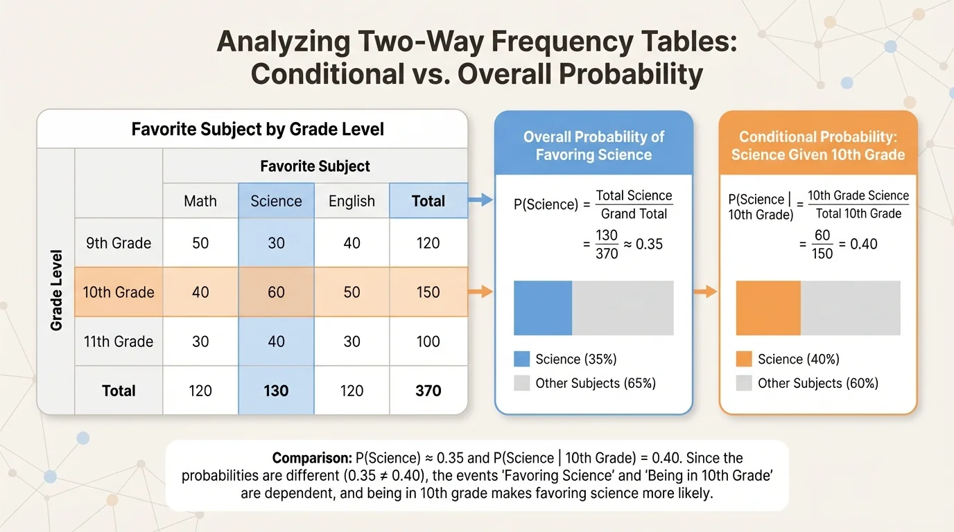
To decide whether two events are independent, we compare a conditional probability with the corresponding overall probability. The comparison in [Figure 3] captures the key idea: if knowing that a student is in tenth grade changes the probability of favoring science, then the events are not independent.
The overall probability of favoring science is
\[P(\textrm{Science}) = \frac{68}{160} = 0.425\]
We already found that
\[P(\textrm{Science} \mid \textrm{Tenth}) = \frac{28}{60} \approx 0.467\]
Because \(0.467 \neq 0.425\), the events "favors science" and "is in tenth grade" are not independent in this sample.
Another way to test independence is to use the multiplication rule for independent events:
\[P(A \cap B) = P(A)P(B)\]
Let \(A\) be "Science" and \(B\) be "Tenth." Then
\[P(A \cap B) = \frac{28}{160} = 0.175\]
while
\[P(A)P(B) = \frac{68}{160} \cdot \frac{60}{160} = 0.425 \cdot 0.375 = 0.159375\]
Since \(0.175 \neq 0.159375\), the events are again shown to be not independent.
If two events are independent, then knowing one event happened does not change the probability of the other. In real survey data, exact independence is uncommon because groups often have different preferences, habits, or characteristics.
Worked example 1
Find the probability that a randomly selected student is a tenth grader who favors science.
Step 1: Identify the joint frequency.
The cell for tenth grade and science contains \(28\).
Step 2: Identify the total number of students.
The grand total is \(160\).
Step 3: Form the probability.
\(P(\textrm{Tenth and Science}) = \dfrac{28}{160} = \dfrac{7}{40} = 0.175\).
The probability is \(0.175\), or \(17.5\%\).
This is a joint probability because it describes both categories at once.
Worked example 2
Find the probability that a randomly selected student is in eleventh grade, given that the student favors math.
Step 1: Restrict the sample space to students who favor math.
The math column total is \(54\).
Step 2: Find how many of those students are eleventh graders.
The eleventh-grade math cell is \(20\).
Step 3: Compute the conditional probability.
\[P(\textrm{Eleventh} \mid \textrm{Math}) = \frac{20}{54} = \frac{10}{27} \approx 0.370\]
The estimated probability is about \(37.0\%\).
Notice that the denominator is not \(160\). Because the condition is "given math," the relevant total is the number of students who favor math.
Worked example 3
Decide whether "favoring English" and "being in ninth grade" are independent.
Step 1: Find the overall probability of favoring English.
\(P(\textrm{English}) = \dfrac{38}{160} = 0.2375\).
Step 2: Find the conditional probability of favoring English given ninth grade.
There are \(10\) ninth graders who favor English out of \(50\) ninth graders, so \(P(\textrm{English} \mid \textrm{Ninth}) = \dfrac{10}{50} = 0.20\).
Step 3: Compare the probabilities.
Since \(0.20 \neq 0.2375\), the probabilities are not equal.
The events are not independent.
As we saw earlier in [Figure 3], testing independence always comes down to checking whether the condition changes the probability. If it does, the events are associated rather than independent.
Two-way tables appear in many areas beyond school surveys. In public health, researchers might compare vaccination status and infection outcome. In sports, analysts may compare shot location and whether the shot was made. In transportation studies, planners may compare mode of travel and arrival time. In each case, the same questions appear: what is the overall probability, what is the conditional probability, and are the variables associated?
Schools can use these ideas too. If a counseling department notices that one grade has an unusually high conditional probability of favoring science, it may decide to expand lab opportunities or advanced elective options for that grade. If another grade strongly favors English, the school might adjust reading programs or writing support.
Association versus independence
When conditional probabilities differ across groups, the variables are associated. That does not automatically prove one variable causes the other. It only shows that the distribution of one variable changes when you know the value of the other.
This distinction is important. A survey can reveal patterns, but it cannot by itself prove why the pattern exists.
One common error is mixing up \(P(\textrm{Science} \mid \textrm{Tenth})\) with \(P(\textrm{Tenth} \mid \textrm{Science})\). These are different probabilities because they use different denominators:
\[P(\textrm{Science} \mid \textrm{Tenth}) = \frac{28}{60}\]
but
\[P(\textrm{Tenth} \mid \textrm{Science}) = \frac{28}{68}\]
They answer different questions. The first asks, "Among tenth graders, how many favor science?" The second asks, "Among science-favoring students, how many are tenth graders?"
Another mistake is using a row total when a column total is needed, or using the grand total when the question is conditional. The wording tells you which total belongs in the denominator.
The layout in [Figure 1] helps prevent that confusion because rows, columns, and totals are visually separated. Meanwhile, the row focus in [Figure 2] reminds us that a condition narrows the sample space before we calculate.
Finally, remember that probabilities estimated from sample data describe the sample exactly and the population approximately. A random sample makes that approximation more trustworthy.