A formula can look short and abstract, but its parameters can tell a surprisingly detailed story. In a function such as \(C(m) = 3m + 8\), the numbers \(3\) and \(8\) are not just symbols on a page: one might represent a charge per mile, and the other might represent a starting fee before any travel occurs. In another function like \(P(t) = 500(1.12)^t\), the numbers describe something completely different: a beginning amount and repeated percentage growth. Learning to interpret parameters means learning to read the hidden meaning inside an equation.
In algebra, a parameter is a constant in a function that helps determine how the function behaves. When a function models a situation, each parameter should connect to the context. This is one of the most powerful ideas in mathematical modeling: equations are not only for calculating answers, but also for describing how the world changes.
Linear function: a function with a constant rate of change, often written as \(f(x) = mx + b\).
Exponential function: a function in which the variable appears in the exponent, often written as \(f(x) = a(b)^x\), where equal changes in \(x\) multiply the output by the same factor.
Initial value: the value of the function when the input is \(0\), if that input makes sense in the context.
If you only use a function to plug in numbers, you miss much of its meaning. Parameters reveal whether a quantity starts high or low, whether it rises or falls, whether it changes by equal differences or equal factors, and how quickly the change happens. For example, in a streaming service plan, one parameter might represent the monthly fee, while another could represent an extra charge for each movie watched. In biology, one parameter might represent the number of bacteria at the start of an experiment, while another represents how much the population multiplies each hour.
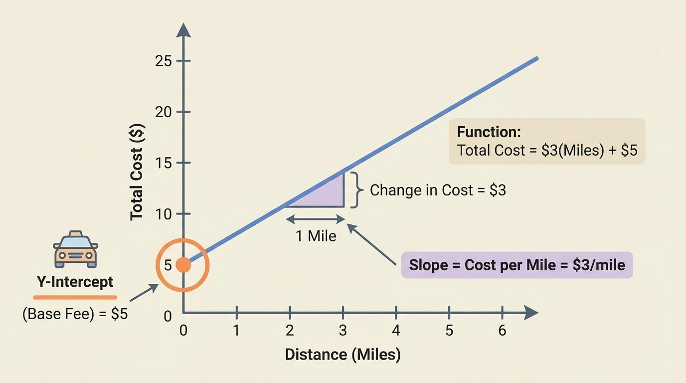
[Figure 1] Interpreting parameters correctly requires attention to rate of change, units, and the meaning of the input variable. If \(t\) measures months, then a growth factor applies each month. If \(x\) measures years, then the same number would mean something very different. Context always decides what a parameter means.
Recall that a function gives exactly one output for each input. Also remember that the graph of a linear function is a straight line, while the graph of an exponential function curves because the outputs change by multiplication rather than by equal differences.
A linear model often has the form \(y = mx + b\). Here, \(m\) is the slope, and \(b\) is the value when \(x = 0\). In context, the slope tells how much the output changes for each increase of \(1\) unit in the input. When \(x = 0\) is meaningful in the situation, this value is the initial value. On a graph, the relationship between these ideas is visible: the y-intercept marks the starting amount, and a slope marker can show the constant increase or decrease per unit of input.
Suppose a taxi company charges a base fee of $8 plus $3 per mile. The total cost \(C\) for \(m\) miles can be written as \(C(m) = 3m + 8\). The parameter \(8\) means the cost starts at $8 even if the taxi goes \(0\) miles. The parameter \(3\) means the cost increases by $3 for each additional mile.
Notice that the units matter. The slope here is not just \(3\); it is \(\$3\) per mile. The initial value is not just \(8\); it is \(\$8\). Without units, interpretation is incomplete.
A linear model can also represent decrease. If a water tank leaks at a steady rate of \(4\) liters per minute and starts with \(120\) liters, then \(W(t) = 120 - 4t\). The initial value \(120\) is the amount of water at time \(0\), and the slope \(-4\) means the amount decreases by \(4\) liters each minute. The negative sign matters: it tells the direction of change.
When reading a linear function, ask two questions: What is the starting amount? and How much does the quantity change for each unit of input? Those two questions usually uncover the meaning of the parameters.
Not every linear function is written in slope-intercept form. You may see descriptions such as "a gym membership costs $25 to join and $15 each month," which leads naturally to \(C(m) = 15m + 25\). You may also see equations written as \(y - 50 = 6(x - 2)\). In this form, the number \(6\) is still the slope, meaning the output changes by \(6\) for each increase of \(1\) in the input.
The numbers \(2\) and \(50\) in \(y - 50 = 6(x - 2)\) tell you that the line passes through the point \((2, 50)\). In context, that point may itself carry meaning. For example, if \(x\) is hours worked and \(y\) is dollars earned, the point could mean that after \(2\) hours, the person has earned $50. Then the slope \(6\) would mean the earnings increase by $6 per additional hour from that point onward.
Linear parameters describe additive change. In a linear function, equal changes in the input produce equal differences in the output. If the slope is \(5\), then each time the input increases by \(1\), the output changes by \(5\). If the input increases by \(10\), the output changes by \(10 \cdot 5 = 50\).
This additive pattern is the key feature of linear models. Whether the slope is positive or negative, the change happens by adding or subtracting the same amount over equal intervals.
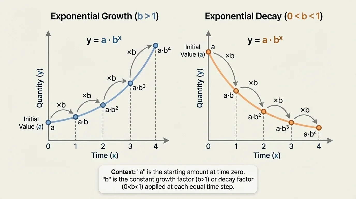
[Figure 2] An exponential model often has the form \(y = a(b)^x\). Here, \(a\) is the initial value, and \(b\) is the growth or decay factor. Unlike a linear function, where the output changes by equal differences, an exponential function changes by equal factors over equal intervals. This pattern appears clearly in graphs: one curve rises more and more steeply, while another falls quickly and then levels off.
Suppose a savings account starts with $500 and grows by \(12\%\) each year. The amount after \(t\) years can be modeled by \(A(t) = 500(1.12)^t\). The parameter \(500\) is the amount at \(t = 0\), so it is the initial amount in the account. The parameter \(1.12\) is the yearly growth factor. It means that each year, the amount is multiplied by \(1.12\).
That multiplier represents a percent increase. Because \(1.12 = 1 + 0.12\), it means a \(12\%\) increase each year. If the model were \(500(0.88)^t\), then \(0.88 = 1 - 0.12\), which would mean a \(12\%\) decrease each year.
For exponential decay, consider a car worth $24,000 that loses \(18\%\) of its value each year. A model is \(V(t) = 24000(0.82)^t\). The parameter \(24{,}000\) is the initial value. The factor \(0.82\) means the car keeps \(82\%\) of its value each year, which is the same as losing \(18\%\) each year.
Exponential functions can feel less intuitive at first because the rate is multiplicative. In a population model, the population might not increase by \(50\) each year; instead, it might increase by \(5\%\) each year. That means the increase itself gets larger over time because the new percentage is taken from a growing amount.
This is why exponential growth can become dramatic. A quantity can begin slowly and then rise sharply. The opposite happens in decay: the quantity drops quickly at first and then decreases more gradually. Later, when comparing models, we return to this visual difference, as shown again in [Figure 2].
Some technologies rely on exponential behavior. Computer storage, viral spread on social networks, and radioactive decay all involve repeated multiplication over equal intervals, even though the contexts are completely different.
Students often confuse the growth factor with the percent rate. The factor and the rate are related, but they are not the same thing. In \(a(1.05)^t\), the factor is \(1.05\), which corresponds to a growth rate of \(5\%\). In \(a(0.93)^t\), the factor is \(0.93\), which corresponds to a decay rate of \(7\%\).
To move from a percent rate to a factor, use these ideas:
For growth at rate \(r\), the factor is \(1 + r\).
For decay at rate \(r\), the factor is \(1 - r\).
Here \(r\) must be written as a decimal. So \(8\% = 0.08\), and the growth factor is \(1.08\). A decay of \(23\%\) means \(r = 0.23\), so the decay factor is \(0.77\).
| Situation | Percent Rate | Factor | Meaning |
|---|---|---|---|
| Growth | \(5\%\) | \(1.05\) | Multiply by \(1.05\) each interval |
| Growth | \(12\%\) | \(1.12\) | Multiply by \(1.12\) each interval |
| Decay | \(7\%\) | \(0.93\) | Keep \(93\%\) each interval |
| Decay | \(18\%\) | \(0.82\) | Keep \(82\%\) each interval |
Table 1. Common connections between percentage change and exponential factors.
Another important detail is the time interval. A model such as \(N(t) = 600(1.04)^t\) means different things depending on whether \(t\) is measured in days, months, or years. The factor applies once per unit of the input variable.
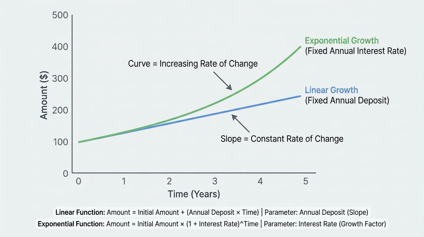
[Figure 3] Linear and exponential functions can sometimes start with the same initial value, but they behave very differently afterward. A line and an exponential curve may begin at the same point and then separate because one changes by equal differences and the other changes by equal factors.
Compare \(L(t) = 100 + 20t\) and \(E(t) = 100(1.2)^t\). Both begin at \(100\) when \(t = 0\). But in the linear model, the amount increases by \(20\) each time. In the exponential model, the amount is multiplied by \(1.2\) each time, which means a \(20\%\) increase each interval.
| Feature | Linear Model | Exponential Model |
|---|---|---|
| General form | \(y = mx + b\) | \(y = a(b)^x\) |
| Initial value | \(b\) | \(a\) |
| Change type | Add the same amount | Multiply by the same factor |
| Parameter meaning | Slope = constant rate | Factor = constant multiplier |
| Typical graph | Straight line | Curve |
Table 2. Comparison of parameter meanings in linear and exponential models.
This distinction matters in real situations. A salary that rises by $2,000 each year is linear. A population that grows by \(2\%\) each year is exponential. The numbers may look similar at first, but they describe different kinds of change.
Now let us interpret parameters carefully in several contexts and connect them to the equations.
Worked example 1
A phone plan costs $20 per month plus $0.10 for each text message sent. The monthly cost is modeled by \(C(n) = 0.10n + 20\), where \(n\) is the number of text messages.
Step 1: Identify the initial value.
The constant term is \(20\), so when \(n = 0\), \(C(0) = 20\).
This means the customer pays $20 even if no texts are sent.
Step 2: Identify the rate of change.
The coefficient of \(n\) is \(0.10\).
This means the cost increases by $0.10 for each text message.
Step 3: State the interpretation clearly in context.
The parameter \(20\) is the monthly base fee, and the parameter \(0.10\) is the charge per text.
The parameters describe a linear model with a starting cost and a constant additional cost per message.
This example shows that in a linear function, the coefficient of the variable often represents a "per unit" cost, speed, or change. The constant term usually represents a beginning amount or fixed fee.
Worked example 2
A town has a population modeled by \(P(t) = 18{,}000(1.03)^t\), where \(t\) is measured in years.
Step 1: Identify the initial value.
The initial value is \(18{,}000\), because \(P(0) = 18{,}000(1.03)^0 = 18{,}000\).
Step 2: Interpret the growth factor.
The factor is \(1.03\). Since \(1.03 = 1 + 0.03\), the population grows by \(3\%\) each year.
Step 3: State the meaning of the parameters in context.
The parameter \(18{,}000\) is the town's population at the start of the model, and \(1.03\) means the population is multiplied by \(1.03\) every year.
This is exponential growth because the amount changes by a constant factor, not by a constant difference.
Notice that if the factor had been \(0.97\), the model would describe a population decreasing by \(3\%\) each year instead.
Worked example 3
A machine's value is modeled by \(V(t) = 7500(0.85)^t\), where \(t\) is in years.
Step 1: Find the initial value.
At \(t = 0\), \(V(0) = 7500\).
So the machine is worth $7,500 at the beginning.
Step 2: Interpret the factor.
The factor is \(0.85\), meaning the machine keeps \(85\%\) of its value each year.
Step 3: Convert the factor to a decay rate.
Because \(1 - 0.85 = 0.15\), the machine loses \(15\%\) of its value each year.
Step 4: Interpret the full model.
The parameter \(7500\) is the initial value, and \(0.85\) is the yearly decay factor.
This is exponential decay because the value is repeatedly multiplied by a factor less than \(1\).
Depreciation is a common real-world use of exponential decay. Cars, electronics, and industrial machines often lose value by a percentage, not by the same number of dollars each year.
Worked example 4
A container holds \(90\) liters of liquid and drains at a steady rate of \(2.5\) liters per minute. Write and interpret a model.
Step 1: Determine the initial amount.
The container starts with \(90\) liters, so the initial value is \(90\).
Step 2: Determine the rate of change.
The amount decreases by \(2.5\) liters each minute, so the slope is \(-2.5\).
Step 3: Write the function.
\[L(t) = 90 - 2.5t\]
Step 4: Interpret the parameters.
The parameter \(90\) means the starting amount of liquid, and \(-2.5\) means the liquid decreases by \(2.5\) liters each minute.
The negative slope tells us the quantity is falling over time.
One frequent mistake is treating the initial value as the value after one time period instead of the value at time \(0\). In \(A(t) = 400(1.08)^t\), the \(400\) is the starting amount, not the amount after one year.
Another mistake is reading an exponential factor as if it were a linear rate. In \(500(1.07)^t\), the number \(1.07\) does not mean "increase by \(1.07\)." It means "multiply by \(1.07\)," which is a \(7\%\) increase each interval.
Students also sometimes ignore units. If a model uses months, then the growth or decay happens monthly. If the model uses hours, then the factor or slope applies every hour. This is why the same parameter can mean very different things in different contexts.
Ask three interpretation questions. When you see a model, ask: What is the input variable and its unit? What is the output variable and its unit? What does each parameter tell me about the starting value or the way the output changes as the input increases?
These questions help prevent misreading and make your interpretation precise instead of vague.
Linear models appear in hourly wages, rental fees, utility charges with a fixed fee plus usage, and distance traveled at constant speed. If a delivery worker earns $18 per hour plus a one-time $25 fixed payment, the earnings model is linear because each added hour contributes the same amount.
Exponential models appear in compound interest, population growth, disease spread under simplified conditions, radioactive decay, and depreciation. In finance, an account balance that gains \(4\%\) every year is naturally exponential because each year's increase depends on the current balance, not just the original deposit.
Scientists and economists pay close attention to parameter interpretation because policy and decisions often depend on it. A growth factor of \(1.02\) may seem small, but when applied repeatedly over many years, it can make a large difference. Likewise, a decay factor of \(0.95\) can slowly reduce a quantity much more than people first expect.
When you look back at the linear graph in [Figure 1] and the model comparison in [Figure 3], the visual difference reinforces the practical one: constant addition creates a straight-line trend, while constant multiplication creates a curved trend that can accelerate or taper.
Interpreting parameters is a modeling skill, not just an algebra skill. It turns equations into descriptions of cost, growth, decline, and change over time. Once you can explain what each number means in words, you are using mathematics the way scientists, engineers, and analysts do.