If you had a huge polynomial like \(p(x)=3x^5-7x^3+2x^2-9x+4\), would you really want to do full polynomial long division every time just to see what happens when dividing by \(x-2\)? The remarkable fact is that you do not need to. One substitution, \(x=2\), gives the remainder immediately. That shortcut is not a trick; it is a deep and useful theorem that connects division, factors, and zeros of polynomials.
Polynomials appear everywhere in algebra, from graphing functions to solving equations and modeling motion. A central question is often: does a polynomial have a particular factor, and where are its zeros? The Remainder Theorem gives a fast answer when the divisor has the form \(x-a\).
Instead of carrying out long division, you can evaluate the polynomial at \(a\). If the result is \(0\), then the divisor fits perfectly with no remainder. That one idea leads directly to the factor test that students use throughout algebra and precalculus.
When one number divides another with no remainder, we say it is a factor. The same idea extends to polynomials: if dividing one polynomial by another gives remainder \(0\), then the divisor is a factor.
You already know a similar pattern from arithmetic. For example, if \(35\) is divided by \(5\), the remainder is \(0\), so \(5\) is a factor of \(35\). With polynomials, the language is similar, but the objects are expressions like \(x-3\) and \(x+2\).
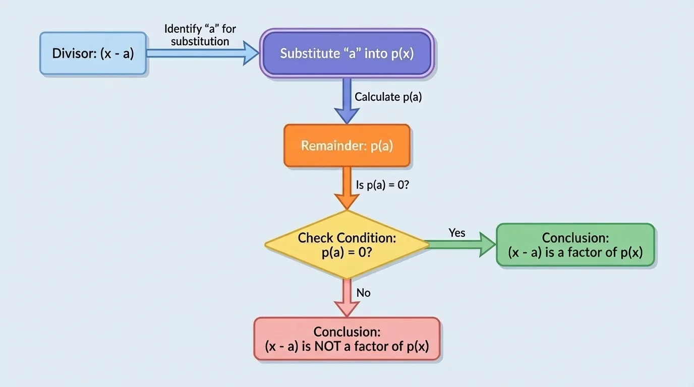
For a polynomial \(p(x)\), the divisor \(x-a\) tells you to look at the number \(a\), as [Figure 1] illustrates. The remainder when \(p(x)\) is divided by \(x-a\) is exactly \(p(a)\).
The theorem is usually written as:
\[\textrm{If } p(x) \textrm{ is divided by } x-a, \textrm{ then the remainder is } p(a).\]
This leads to an equally important statement called the Factor Theorem:
\[(x-a) \textrm{ is a factor of } p(x) \iff p(a)=0.\]
That means two facts are really the same fact viewed from different angles. If \(p(a)=0\), then dividing by \(x-a\) leaves no remainder, so \(x-a\) is a factor. If \(x-a\) is a factor, then the remainder must be \(0\), so \(p(a)=0\).
Zero of a polynomial: a value \(a\) for which \(p(a)=0\).
Factor of a polynomial: an expression that divides the polynomial with remainder \(0\).
Remainder: what is left after division if the division is not exact.
A zero is often also called a root or solution of the equation \(p(x)=0\). If \(a\) is a zero, then \(x-a\) is a factor. This is one of the key relationships in polynomial algebra.
The theorem becomes more believable when you see the algebra behind it. If a polynomial \(p(x)\) is divided by \(x-a\), then division tells us there must be some quotient \(q(x)\) and some remainder \(r\), where the remainder is just a constant because the divisor has degree \(1\).
So we can write
\[p(x)=(x-a)q(x)+r.\]
Now substitute \(x=a\). The term \((x-a)q(x)\) becomes \((a-a)q(a)=0\), so
\(p(a)=r.\)
That is exactly the Remainder Theorem. The remainder is not mysterious; it is simply the value of the polynomial at \(a\).
To find the remainder on division by \(x-a\), substitute \(a\) into the polynomial. Be careful with signs. If the divisor is \(x-4\), then use \(a=4\). If the divisor is \(x+4\), rewrite it as \(x-(-4)\), so use \(a=-4\).
Worked example 1
Find the remainder when \(p(x)=2x^3-5x^2+x+7\) is divided by \(x-3\).
Step 1: Identify \(a\)
The divisor is \(x-3\), so \(a=3\).
Step 2: Evaluate \(p(3)\)
Substitute \(x=3\):
\(p(3)=2(3)^3-5(3)^2+3+7\).
Step 3: Simplify
\(p(3)=2(27)-5(9)+3+7=54-45+3+7=19\).
The remainder is \(19\).
Notice how much faster this is than full long division. The theorem turns a division question into a substitution question.
It also works for negative values and fractions. For example, if dividing by \(x+2\), you evaluate at \(x=-2\). If dividing by \(x-\dfrac{1}{2}\), you evaluate at \(x=\dfrac{1}{2}\).
Worked example 2
Find the remainder when \(f(x)=x^4-3x+8\) is divided by \(x+2\).
Step 1: Identify \(a\)
Since \(x+2=x-(-2)\), we use \(a=-2\).
Step 2: Evaluate \(f(-2)\)
\(f(-2)=(-2)^4-3(-2)+8\).
Step 3: Simplify
\(f(-2)=16+6+8=30\).
The remainder is \(30\).
The factor question is one of the most powerful uses of the theorem. To test whether \((x-a)\) is a factor of \(p(x)\), compute \(p(a)\). If \(p(a)=0\), then yes. If \(p(a)\neq 0\), then no.
This matters because factoring polynomials often begins by searching for likely zeros. Each successful test gives you a linear factor, which can then be used to reduce the polynomial and continue factoring.
Worked example 3
Determine whether \(x-2\) is a factor of \(p(x)=x^3-4x^2+x+6\).
Step 1: Evaluate \(p(2)\)
\(p(2)=2^3-4(2^2)+2+6=8-16+2+6\).
Step 2: Simplify
\(p(2)=8-16+8=0\).
Step 3: Interpret the result
Because \(p(2)=0\), the remainder is \(0\). Therefore \(x-2\) is a factor of the polynomial.
The theorem confirms the factor immediately.
If the result had been anything other than \(0\), the divisor would not be a factor. This makes the theorem an efficient screening tool.
[Figure 2] The connection between algebra and graphs becomes much clearer here. A zero of \(p(x)\) is a value \(a\) such that \(p(a)=0\), and on the graph this means the point \((a,0)\) lies on the x-axis.
If \(a\) is a zero, then \(x-a\) is a factor. If \(x-a\) is a factor, then \(a\) is a zero. So when you solve \(p(x)=0\), you are really finding the values that make the polynomial divisible by certain linear factors.
For example, if \(p(x)=(x-1)(x+2)(x-4)\), then the zeros are \(1\), \(-2\), and \(4\). The graph crosses or touches the x-axis at those x-values.
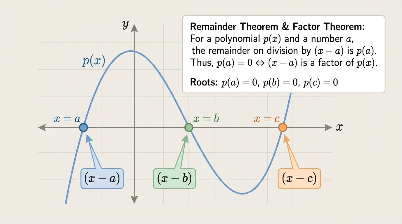
This is why the theorem is so useful in graphing. Once you know a factor, you know a zero; once you know a zero, you know where the graph meets the x-axis.
Engineers and scientists often use polynomial models because they are flexible and easy to evaluate on computers. Quick factor and remainder checks help verify whether a model behaves as expected at special input values.
Later, when you study higher-degree polynomials, this link becomes even more important. A complicated graph can often be understood by identifying zeros and corresponding factors.
The next examples combine several ideas: substitution, factor testing, and solving for unknown constants.
Worked example 4
Determine whether \(x+1\) is a factor of \(g(x)=2x^4-3x^2+5x-4\).
Step 1: Match the divisor to \(x-a\)
Since \(x+1=x-(-1)\), use \(a=-1\).
Step 2: Evaluate \(g(-1)\)
\(g(-1)=2(-1)^4-3(-1)^2+5(-1)-4\).
Step 3: Simplify carefully
\(g(-1)=2(1)-3(1)-5-4=2-3-5-4=-10\).
Step 4: Decide
Because \(g(-1)=-10\neq 0\), the remainder is \(-10\), so \(x+1\) is not a factor.
This example shows how sign mistakes can change the answer, so substitute carefully.
Now consider a common algebra task: choosing a constant so that a given binomial becomes a factor.
Worked example 5
Find the value of \(k\) so that \(x-3\) is a factor of \(p(x)=x^3+kx^2-5x+6\).
Step 1: Use the factor condition
If \(x-3\) is a factor, then \(p(3)=0\).
Step 2: Substitute \(x=3\)
\(p(3)=3^3+k(3^2)-5(3)+6=27+9k-15+6\).
Step 3: Simplify
\(p(3)=18+9k\).
Step 4: Set equal to \(0\) and solve
Because \(p(3)=0\), we get \(18+9k=0\). So \(9k=-18\), and \(k=-2\).
The required value is \(k=-2\).
This method is much more efficient than trying to factor the expression first. The theorem turns the problem into a simple equation.
Worked example 6
The remainder when \(h(x)=x^3-2x^2+mx+5\) is divided by \(x-1\) is \(7\). Find \(m\).
Step 1: Apply the Remainder Theorem
The remainder on division by \(x-1\) is \(h(1)\), so \(h(1)=7\).
Step 2: Evaluate \(h(1)\)
\(h(1)=1^3-2(1)^2+m(1)+5=1-2+m+5\).
Step 3: Simplify and solve
\(h(1)=m+4\). Since \(h(1)=7\), we have \(m+4=7\), so \(m=3\).
The value of \(m\) is \(3\).
One frequent error is using the wrong sign. If the divisor is \(x+5\), students sometimes substitute \(5\) instead of \(-5\). Always rewrite mentally as \(x-(-5)\).
Another mistake is thinking that \(p(a)\) gives the quotient. It does not. It gives only the remainder. The quotient is a different polynomial.
A third mistake is failing to use parentheses when substituting negative values. For example, in \(x^3-4x\), evaluating at \(x=-2\) must be written as \((-2)^3-4(-2)\), not \(-2^3-4-2\).
The sign pattern in factors also matters. If \(a=3\), the factor is \(x-3\), not \(x+3\). If \(a=-3\), the factor is \(x+3\). As we saw earlier in [Figure 1], the number substituted is the opposite of the constant term in the binomial \(x-a\).
In mathematical modeling, a polynomial can represent height, profit, population trend, or signal behavior over time. Testing whether \(p(a)=0\) checks whether the model predicts an output of \(0\) at input \(a\). That can matter when identifying break-even points, moments of impact, or equilibrium values.
For example, in physics, the height of an object might be modeled by a polynomial approximation over a short time interval. If \(h(t)=0\) for some value of \(t\), then the object is on the ground at that moment. The corresponding factor \(t-a\) reflects that zero of the model.
In graphing technology and computer algebra systems, substitution is also the fastest way to test a potential zero before doing more complicated algebra. This is one reason the theorem is used so often in both hand calculations and software.
When analyzing graphs, the x-intercepts identified from factors help you predict turning behavior and overall shape. The visual pattern of roots on the graph, as shown earlier in [Figure 2], is directly connected to the algebraic factorization.
[Figure 3] The Remainder Theorem connects naturally to synthetic division, a quick procedure for dividing by \(x-a\). Synthetic division uses the number \(a\), and its final value is the same remainder \(p(a)\).
For instance, if you test \(x-2\), synthetic division uses the number \(2\). The last number in the synthetic division row is the remainder, and it must match the value obtained by direct substitution.
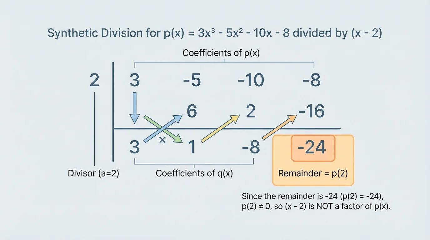
This means you have two efficient tools: direct evaluation and synthetic division. Direct evaluation is often best for a quick remainder or factor test. Synthetic division is especially useful once you know a factor and want to reduce the polynomial to a lower degree.
The theorem also supports a broader strategy for factoring. You test possible zeros, confirm one with \(p(a)=0\), divide out the factor, and then continue factoring the quotient. This step-by-step reduction is a core method in polynomial algebra.
"A zero is not just a number where the function equals zero; it is also the key that unlocks a factor."
That idea captures why the theorem is so powerful. It ties together function values, division, factors, and graphs in one compact principle.