Airline schedules, game graphics, phone networks, and economic models all depend on solving many equations at once. Writing each equation separately works for small problems, but for larger systems, mathematicians and scientists use a more powerful language: matrices. A whole system can be compressed into one clean statement, and that compact form makes advanced solving methods possible.
When you already know how to solve a system of equations by graphing, substitution, or elimination, the next step is learning how to organize the system. That organization matters. A matrix equation keeps the same mathematical information, but it arranges it in a form that is easier to analyze, solve, and use with technology.
A system of linear equations is a collection of equations that share the same variables. For example, the system consisting of \(2x + 3y = 7\) and \(x - y = 4\) asks for values of \(x\) and \(y\) that satisfy both equations at the same time. Instead of seeing this as two separate lines of algebra, we can view it as one structure.
That structure is especially useful when there are many variables. A scientist may track several unknown quantities at once, and writing one matrix equation is much more efficient than repeating every equation separately. The matrix form also prepares you for methods such as using inverses, determinants, and row operations.
To write a system as a matrix equation, each equation should first be written in standard linear form, with all variable terms on one side and constants on the other. The variables must appear in the same order in every equation, such as \(x, y, z\).
If the variables are not arranged consistently, the matrix entries will not match the correct variables. This is one of the most common mistakes students make when first learning matrix form.
Consider the system
\[\begin{aligned}2x+3y&=7\x-y&=4\end{aligned}\]
This system contains three important pieces of information. First, the coefficients are the numbers multiplying the variables: \(2\), \(3\), \(1\), and \(-1\). Second, the variables are \(x\) and \(y\). Third, the constants on the right side are \(7\) and \(4\).
If we group those pieces carefully, we can place the coefficients into a rectangular array, the variables into a column, and the constants into another column. This is the idea behind matrix form.
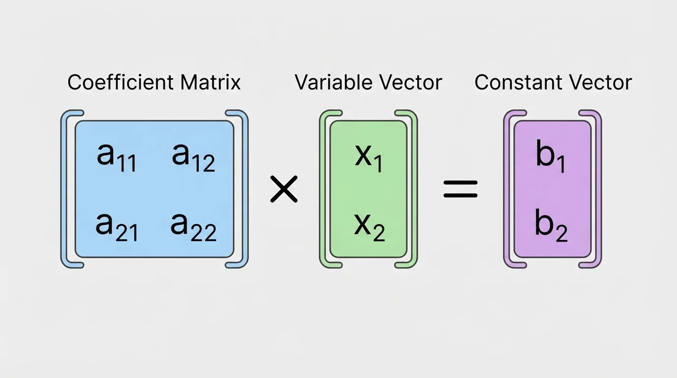
A matrix is a rectangular array of numbers arranged in rows and columns.
A variable vector is a column vector whose entries are the variables of the system, such as \(\begin{bmatrix}x\y\end{bmatrix}\).
A coefficient matrix is the matrix formed by the coefficients of the variables in the system.
[Figure 1] The system above can be reorganized without changing its meaning. We are not solving yet; we are rewriting. The goal is to express the same relationships in a compact algebraic form.
A whole system can be packed into a single expression by writing \(A\mathbf{x}=\mathbf{b}\), where \(A\) is the coefficient matrix, \(\mathbf{x}\) is the variable vector, and \(\mathbf{b}\) is the constant vector. For the system above, we write
\[\begin{bmatrix}2&3\\1&-1\end{bmatrix}\begin{bmatrix}x\y\end{bmatrix}=\begin{bmatrix}7\\4\end{bmatrix}\]
Here, the matrix \(A=\begin{bmatrix}2&3\\1&-1\end{bmatrix}\), the variable vector is \(\mathbf{x}=\begin{bmatrix}x\y\end{bmatrix}\), and the constant vector is \(\mathbf{b}=\begin{bmatrix}7\\4\end{bmatrix}\).
This notation looks different from a familiar system, but it says exactly the same thing. It is just a more structured way to store the information.
In general, if a system has \(m\) equations and \(n\) variables, then the coefficient matrix has size \(m \times n\). The variable vector has size \(n \times 1\), and the constant vector has size \(m \times 1\).
[Figure 2] The compact form still contains every original equation through row-by-column multiplication. When a matrix multiplies a variable vector, each row of the matrix combines with the variable entries to produce one equation.
For example,
\[\begin{bmatrix}2&3\\1&-1\end{bmatrix}\begin{bmatrix}x\y\end{bmatrix}=\begin{bmatrix}2x+3y\x-y\end{bmatrix}\]
The first row \((2,3)\) produces \(2x+3y\). The second row \((1,-1)\) produces \(x-y\). Setting that result equal to \(\begin{bmatrix}7\\4\end{bmatrix}\) gives the original system back.
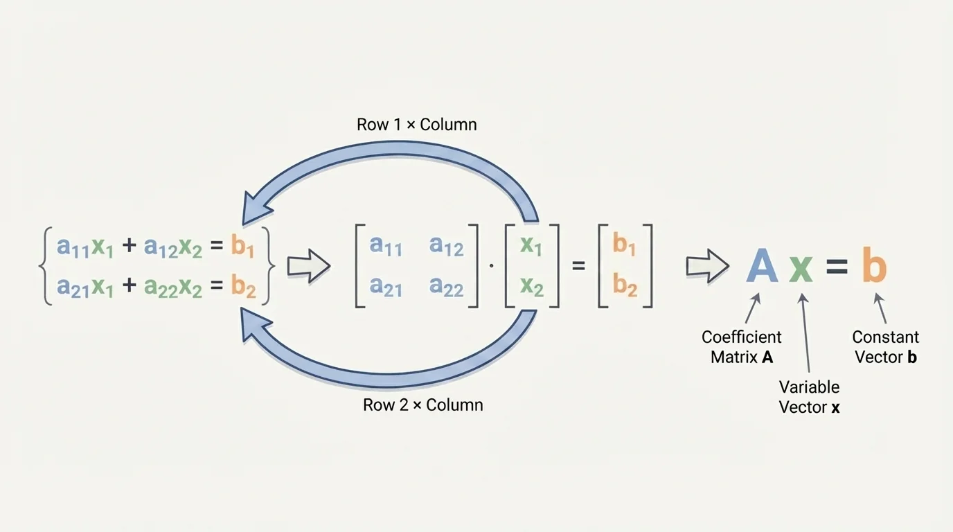
This is why matrix form is so useful: the rows preserve equations, and the columns preserve which coefficient belongs to which variable. As we saw in [Figure 1], the organization is not random. Every entry has a precise role.
Why order matters
If the variable vector is \(\begin{bmatrix}x\y\end{bmatrix}\), then the first column of the coefficient matrix must contain all coefficients of \(x\), and the second column must contain all coefficients of \(y\). If you switch the variable order to \(\begin{bmatrix}y\x\end{bmatrix}\), then the coefficient columns must also switch.
That means matrix form depends on consistency. The same variables, in the same order, must appear throughout the system.
Here is a reliable method for converting a system to matrix form.
Step 1: Write every equation in standard linear form, with variables on the left and constants on the right.
Step 2: Choose an order for the variables, such as \(x, y\) or \(x, y, z\).
Step 3: Read off the coefficients row by row to form the coefficient matrix.
Step 4: Write the variable vector using the chosen order.
Step 5: Write the constants in a column vector on the right side.
If a variable is missing from one equation, its coefficient is \(0\). For example, \(3x + y = 5\) and \(2y = 8\) should be treated as \(3x + y = 5\) and \(0x + 2y = 8\).
Convert the system \(3x - 2y = 5\) and \(x + 4y = -1\) into a matrix equation.
Worked example 1
Step 1: Identify the coefficients.
From \(3x - 2y = 5\), the coefficients are \(3\) and \(-2\). From \(x + 4y = -1\), the coefficients are \(1\) and \(4\).
Step 2: Build the coefficient matrix.
\[A=\begin{bmatrix}3&-2\\1&4\end{bmatrix}\]
Step 3: Write the variable vector and constant vector.
\(\mathbf{x}=\begin{bmatrix}x\y\end{bmatrix}\) and \(\mathbf{b}=\begin{bmatrix}5\\-1\end{bmatrix}\).
Step 4: Write the matrix equation.
\[\begin{bmatrix}3&-2\\1&4\end{bmatrix}\begin{bmatrix}x\y\end{bmatrix}=\begin{bmatrix}5\\-1\end{bmatrix}\]
This single equation represents the entire system.
Notice that the coefficients are placed by row, not by equation name or by visual spacing. The first row comes from the first equation, and the second row comes from the second equation.
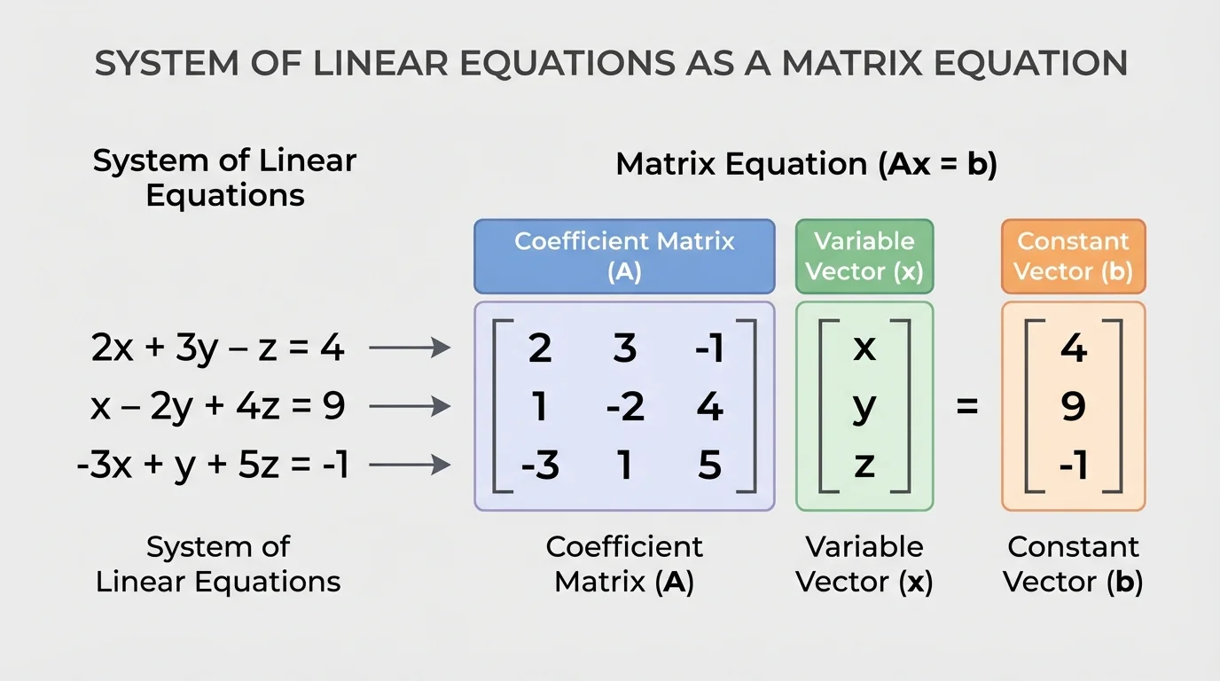
[Figure 3] With three variables, careful alignment becomes even more important. It illustrates how each equation contributes one row while each variable keeps its own column. Convert the system
\[\begin{aligned}x+2y-z&=4\\3x-y+5z&=2\\2x+4y+z&=9\end{aligned}\]
into a matrix equation.
Worked example 2
Step 1: Choose the variable order \(x, y, z\).
This means column \(1\) is for \(x\), column \(2\) is for \(y\), and column \(3\) is for \(z\).
Step 2: Record the coefficients row by row.
The rows are \((1,2,-1)\), \((3,-1,5)\), and \((2,4,1)\).
Step 3: Form the vectors.
\(\mathbf{x}=\begin{bmatrix}x\y\z\end{bmatrix}\) and \(\mathbf{b}=\begin{bmatrix}4\\2\\9\end{bmatrix}\).
Step 4: Write the final matrix equation.
\[\begin{bmatrix}1&2&-1\\3&-1&5\\2&4&1\end{bmatrix}\begin{bmatrix}x\y\z\end{bmatrix}=\begin{bmatrix}4\\2\\9\end{bmatrix}\]
The matrix equation is a compact version of the full three-equation system.
Later, when methods such as row reduction are used, this organized form becomes extremely helpful. One wrong coefficient placement would change the system itself.
This example is where students often realize why matrix form requires careful organization. Convert the system
\[\begin{aligned}y+2x&=6\\3z-x&=4\y-z&=1\end{aligned}\]
into a matrix equation using the variable order \(x, y, z\).
Worked example 3
Step 1: Rewrite each equation in the chosen variable order.
\(2x+y+0z=6\), \(-x+0y+3z=4\), and \(0x+y-z=1\).
Step 2: Form the coefficient matrix.
\[A=\begin{bmatrix}2&1&0\\-1&0&3\\0&1&-1\end{bmatrix}\]
Step 3: Write the variable and constant vectors.
\(\mathbf{x}=\begin{bmatrix}x\y\z\end{bmatrix}\) and \(\mathbf{b}=\begin{bmatrix}6\\4\\1\end{bmatrix}\).
Step 4: State the matrix equation.
\[\begin{bmatrix}2&1&0\\-1&0&3\\0&1&-1\end{bmatrix}\begin{bmatrix}x\y\z\end{bmatrix}=\begin{bmatrix}6\\4\\1\end{bmatrix}\]
The zeros are essential because they show that some variables are absent from particular equations.
A missing variable does not mean "leave a blank." It means the coefficient is exactly \(0\). That zero preserves the correct column structure.
Many computer programs solve systems with thousands or even millions of variables. In those settings, storing equations in matrix form is not just convenient; it is necessary.
This is one reason matrix notation matters far beyond a classroom exercise. It is the language of large-scale computation.
Writing a system as \(A\mathbf{x}=\mathbf{b}\) does not guarantee that the system has exactly one solution. The system may have one solution, no solution, or infinitely many solutions. The matrix form simply represents the system clearly.
For example, if two equations describe the same line, the system may have infinitely many solutions. If two equations are inconsistent, the system may have no solution. If they intersect once, there is one solution. Matrix form can represent all three situations.
| System behavior | Meaning in equations | Meaning in matrix form |
|---|---|---|
| One solution | The equations are consistent and determine a single point | \(A\mathbf{x}=\mathbf{b}\) has one vector solution |
| No solution | The equations are inconsistent | \(A\mathbf{x}=\mathbf{b}\) has no vector solution |
| Infinitely many solutions | At least one equation depends on others | \(A\mathbf{x}=\mathbf{b}\) has many vector solutions |
Table 1. Types of solution behavior for a system and their interpretation in matrix form.
So the matrix equation is a representation, not a promise. Its job is to encode the system faithfully.
You should also be able to go backward. Suppose you are given
\[\begin{bmatrix}4&-2\\3&5\end{bmatrix}\begin{bmatrix}x\y\end{bmatrix}=\begin{bmatrix}8\\1\end{bmatrix}\]
Multiplying row by column gives the system
\[\begin{aligned}4x-2y&=8\\3x+5y&=1\end{aligned}\]
This reverse interpretation is important because textbooks, calculators, and computer software often present systems directly in matrix form.
Suppose a concert venue sells regular tickets and premium tickets. If \(x\) is the number of regular tickets and \(y\) is the number of premium tickets, then different conditions can produce a system such as \(x+y=500\) and \(25x+40y=16{,}000\). In matrix form, this becomes
\[\begin{bmatrix}1&1\\25&40\end{bmatrix}\begin{bmatrix}x\y\end{bmatrix}=\begin{bmatrix}500\\16000\end{bmatrix}\]
Economists and event planners like this form because it packages the constraints neatly and supports fast computation.
In chemistry and manufacturing, mixture problems also lead to systems. If two solutions are combined to produce a target concentration, the unknown amounts can be placed into a variable vector, while the concentration relationships become the rows of a coefficient matrix.
Engineers use matrix equations to model forces, currents, and network connections. Even when the underlying story changes, the mathematical structure stays recognizable: coefficients in a matrix, unknowns in a vector, outcomes in another vector.
Why matrices help solve systems
Once a system is written as \(A\mathbf{x}=\mathbf{b}\), new tools become available. If the matrix \(A\) has an inverse, the solution can be written as \(\mathbf{x}=A^{-1}\mathbf{b}\). Even when inverses are not practical, row operations and augmented matrices build directly on this organized representation.
That is the deeper reason for learning matrix equations: they are not just shorter notation. They open the door to efficient methods for solving and analyzing systems.
Keep these rules in mind whenever you represent a system as a matrix equation:
First, every equation must use the same variable order.
Second, use \(0\) for any missing variable.
Third, the coefficient matrix contains only coefficients, not variables or constants.
Fourth, the variable vector contains only variables.
Fifth, the constant vector contains the right-side constants.
When those rules are followed, the matrix equation \(A\mathbf{x}=\mathbf{b}\) is an exact translation of the original system. And once the system is in that form, it is ready for more advanced algebraic tools.