A weather app says there is a \(40\%\) chance of rain tomorrow. But if you also learn that a storm front is moving in, that probability may jump sharply. The event has not changed, but the information has. That is the central idea of conditional probability: probabilities can shift when we know something else has happened.
In probability, we often study how events are related. Sometimes one event makes another more likely. Sometimes it makes it less likely. And sometimes it changes nothing at all. When it changes nothing, we call the events independent. These ideas are essential in fields such as medicine, economics, sports analytics, and engineering because decisions are often based not just on raw probability, but on probability given evidence.
An event is a set of outcomes. If event \(A\) is "a student is in the music club" and event \(B\) is "the student plays a sport," then the probability \(P(A)\) means the chance a randomly chosen student is in the music club. But \(P(A\mid B)\) means something more specific: the chance the student is in the music club given that the student already plays a sport.
That phrase "given that" is crucial. It means we are no longer looking at the whole group. We are looking only at the outcomes inside event \(B\). In other words, event \(B\) becomes the new sample space. This shift is why conditional probability can be very different from ordinary probability.
Recall that \(P(A\cap B)\) means the probability that both events happen. The symbol \(\cap\) means "and" or "intersection." Also remember that probabilities are between \(0\) and \(1\), inclusive.
If knowing \(B\) has happened changes the probability of \(A\), then the events are related in some way. For example, if \(A\) is "a person has a cough" and \(B\) is "a person has a respiratory infection," then \(P(A\mid B)\) is usually much larger than \(P(A)\). The condition gives useful information.
Conditional probability is the probability that event \(A\) occurs given that event \(B\) has already occurred.
When \(P(B)>0\), the conditional probability of \(A\) given \(B\) is
\[P(A\mid B)=\frac{P(A\cap B)}{P(B)}\]
This formula says: take the probability that both \(A\) and \(B\) happen, then divide by the probability of the condition event \(B\).
The denominator is \(P(B)\) because once we know \(B\) happened, the outcomes outside \(B\) are no longer relevant. We are zooming in on only the part of the sample space where \(B\) is true.
The formula only makes sense when \(P(B)>0\). If \(P(B)=0\), then event \(B\) never happens, so there is no meaningful group of outcomes on which to condition.
There is also a matching formula in the other direction:
\[P(B\mid A)=\frac{P(A\cap B)}{P(A)}\]
Notice that switching the order changes the denominator. In general, \(P(A\mid B)\) and \(P(B\mid A)\) are not equal. That is one of the most common mistakes students make.
Conditional probability becomes especially clear in a two-way table, as [Figure 1] shows. A table can separate data into categories, and conditional probability asks you to focus on only one row or one column as the new total.
Suppose a school surveys students about whether they are in a club and whether they play a sport. To find \(P(\textrm{club}\mid\textrm{sport})\), you do not divide by the total number of students in the survey. You divide by the number of students who play a sport, because those are the only students in the conditioned group.
| Group | In a club | Not in a club | Total |
|---|---|---|---|
| Play a sport | \(48\) | \(32\) | \(80\) |
| Do not play a sport | \(27\) | \(43\) | \(70\) |
| Total | \(75\) | \(75\) | \(150\) |
Table 1. Student counts organized by sports participation and club membership.
From this table, \(P(\textrm{club})=\dfrac{75}{150}=\dfrac{1}{2}\). But \(P(\textrm{club}\mid\textrm{sport})=\dfrac{48}{80}=\dfrac{3}{5}\). These are different because the second probability uses a smaller sample space: only students who play a sport.
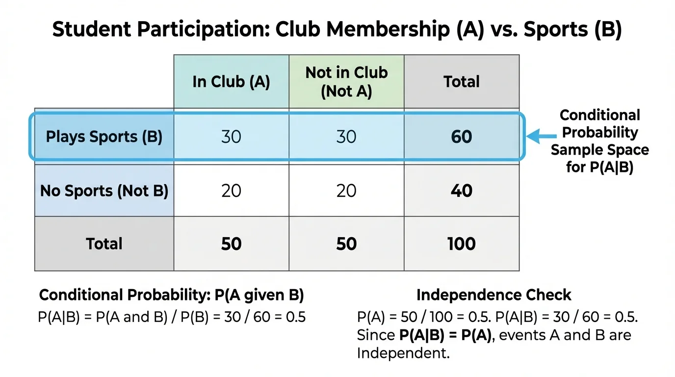
That shift in the denominator is the heart of conditional probability. Instead of asking, "Out of everyone, how many are in a club?" we ask, "Out of the students who play a sport, how many are in a club?"
This table also shows why wording matters. If you reverse the condition, then \(P(\textrm{sport}\mid\textrm{club})=\dfrac{48}{75}\), which is not the same as \(\dfrac{48}{80}\). The intersection stays the same, but the condition changes the total you divide by.
Worked example
Using Table 1, find \(P(\textrm{sport}\mid\textrm{club})\).
Step 1: Identify the condition.
The phrase "given club" means we look only at students who are in a club. From the table, there are \(75\) such students.
Step 2: Find how many satisfy both conditions.
The number of students who are in a club and play a sport is \(48\).
Step 3: Form the conditional probability.
\(P(\textrm{sport}\mid\textrm{club})=\dfrac{48}{75}=\dfrac{16}{25}=0.64\).
The probability is
\[P(\textrm{sport}\mid\textrm{club})=0.64\]
So, among students in a club, \(64\%\) play a sport.
Notice how the denominator came from the condition. That is the reliable question to ask yourself every time: What group am I restricted to?
The same idea works with percentages, fractions, or large data sets. Whether the data come from a classroom survey or a hospital database, conditional probability always means "inside the condition group."
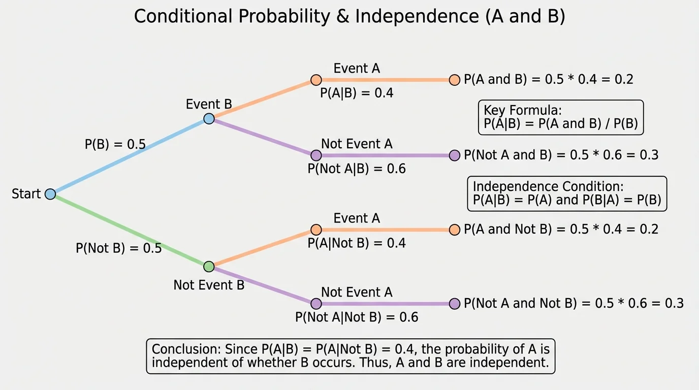
Independence is one of the most elegant ideas in probability, and [Figure 2] illustrates it well: if learning that \(B\) happened does not change the probability of \(A\), then \(A\) and \(B\) are independent. In symbols, that means
\[P(A\mid B)=P(A)\]
provided that \(P(B)>0\).
There is a matching statement in the other direction. If learning that \(A\) happened does not change the probability of \(B\), then
\[P(B\mid A)=P(B)\]
provided that \(P(A)>0\).
For independent events, both statements are true. Intuitively, the events do not influence each other. One event gives no extra information about the other.
Using the conditional probability formula, we can connect independence to another important equation. If \(A\) and \(B\) are independent, then
\[P(A\cap B)=P(A)P(B)\]
Here is why. Start from \(P(A\mid B)=\dfrac{P(A\cap B)}{P(B)}\). If \(A\) and \(B\) are independent, then \(P(A\mid B)=P(A)\). So \(\dfrac{P(A\cap B)}{P(B)}=P(A)\), and multiplying both sides by \(P(B)\) gives \(P(A\cap B)=P(A)P(B)\).
This product rule is often the fastest way to test independence when you already know \(P(A)\), \(P(B)\), and \(P(A\cap B)\). Later, when interpreting real data, keep in mind what [Figure 2] emphasizes: the proportion for event \(A\) stays the same even after we restrict attention to event \(B\).
What independence really means
Independent events are not required to have the same probability, and they are not required to have no overlap. They may overlap a lot or a little. Independence only means that knowledge of one event does not change the probability of the other.
A classic example is flipping a coin and rolling a die. Let \(A\) be "the coin lands heads" and \(B\) be "the die shows an even number." Then \(P(A)=\dfrac{1}{2}\), \(P(B)=\dfrac{1}{2}\), and \(P(A\cap B)=\dfrac{1}{4}\). Since \(\dfrac{1}{4}=\dfrac{1}{2}\cdot\dfrac{1}{2}\), the events are independent.
Worked example
A single card is drawn from a standard deck of \(52\) cards. Let \(A\) be "the card is a heart" and \(B\) be "the card is a face card." Are \(A\) and \(B\) independent?
Step 1: Find \(P(A)\).
There are \(13\) hearts in the deck, so \(P(A)=\dfrac{13}{52}=\dfrac{1}{4}\).
Step 2: Find \(P(B)\).
There are \(12\) face cards total: jacks, queens, and kings. So \(P(B)=\dfrac{12}{52}=\dfrac{3}{13}\).
Step 3: Find \(P(A\cap B)\).
The heart face cards are jack of hearts, queen of hearts, and king of hearts, so there are \(3\) such cards. Thus \(P(A\cap B)=\dfrac{3}{52}\).
Step 4: Compare with the product \(P(A)P(B)\).
\(P(A)P(B)=\dfrac{1}{4}\cdot\dfrac{3}{13}=\dfrac{3}{52}\).
Because \(P(A\cap B)=P(A)P(B)\), the events are independent.
This can also be checked using conditional probability. Since \(P(A\mid B)=\dfrac{3/52}{12/52}=\dfrac{3}{12}=\dfrac{1}{4}=P(A)\), knowing the card is a face card does not change the chance that it is a heart.
That result may feel surprising at first, which is one reason independence is worth studying carefully. Some pairs of events seem related, but the probabilities reveal whether the relationship is real.
Conditional probability becomes especially important when interpreting medical tests. A test result is one event, and having a disease is another. Doctors and researchers constantly ask questions such as "What is the probability a patient has the disease given a positive test?"
Worked example
In a screening program for \(1{,}000\) people, \(80\) people have a certain condition. Of those \(80\), \(68\) test positive. Of the \(920\) people without the condition, \(92\) test positive. Find \(P(\textrm{condition}\mid\textrm{positive})\).
Step 1: Find the number of positive tests.
Positive tests come from two groups: \(68\) true positives and \(92\) false positives. So the total number of positive tests is \(68+92=160\).
Step 2: Find the number with both the condition and a positive test.
That number is \(68\).
Step 3: Form the conditional probability.
\(P(\textrm{condition}\mid\textrm{positive})=\dfrac{68}{160}=\dfrac{17}{40}=0.425\).
The probability is
\[P(\textrm{condition}\mid\textrm{positive})=0.425\]
So a person who tests positive has a \(42.5\%\) chance of actually having the condition in this data set.
This example shows why conditional probability matters more than intuition. Even if a test catches many real cases, the probability of having the disease given a positive test may still be much lower than expected if false positives also occur often.
It also shows that the events "has the condition" and "tests positive" are not independent. If they were independent, the positive result would not change the probability of having the condition. But here, \(P(\textrm{condition})=\dfrac{80}{1000}=0.08\), while \(P(\textrm{condition}\mid\textrm{positive})=0.425\), which is much larger.
Medical researchers, data scientists, and quality-control engineers all rely on conditional probability because raw percentages can be misleading when the population is divided into important subgroups.
Several ideas in this topic look similar but mean different things, and [Figure 3] helps separate two of the most commonly confused relationships. Careful reading of notation and context is essential.
First, \(P(A\mid B)\) is not usually the same as \(P(B\mid A)\). For example, the probability that a student is left-handed given that the student plays tennis is not the same as the probability that a student plays tennis given that the student is left-handed. The same two events are involved, but the conditioning group changes.
Second, mutually exclusive events are not the same as independent events. Mutually exclusive events cannot happen together, so \(P(A\cap B)=0\). If both events have positive probability, then that cannot equal \(P(A)P(B)\), so the events are not independent.
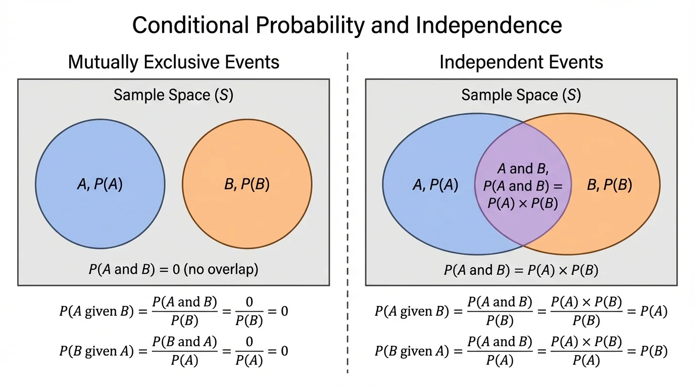
For instance, when rolling one die, let \(A\) be "the result is even" and \(B\) be "the result is odd." These are mutually exclusive because no roll is both even and odd. But they are not independent, because if you know the result is even, then the probability it is odd becomes \(0\), not \(P(B)=\dfrac{1}{2}\).
Third, a conditional probability is undefined if the condition has probability \(0\). You cannot calculate \(P(A\mid B)\) by dividing by \(0\). In practical terms, if event \(B\) never occurs, there is no restricted group to examine.
Finally, independence is about probability, not cause. Two events can be dependent without one causing the other, and two events can be independent even if they happen in the same setting. What matters is whether knowing one event changes the probability of the other. That distinction is easier to keep in mind if you compare the two visual cases in [Figure 3].
In sports, analysts ask questions such as the probability a basketball player makes a shot given that the defender is within a certain distance. In economics, a researcher may study the probability of loan default given a borrower's income bracket. In meteorology, scientists examine the probability of flooding given a specific pattern of rainfall.
Manufacturing provides another powerful example. Suppose event \(A\) is "a product is defective" and event \(B\) is "it was made on machine \(2\)." Then \(P(A\mid B)\) helps identify whether machine \(2\) has a quality problem. If \(P(A\mid B)\) is much larger than \(P(A)\), that suggests products from that machine need closer inspection.
Survey data also depend heavily on conditional probability. A political poll may report the probability a voter supports a policy given age group, region, or education level. These conditional probabilities often reveal patterns hidden by overall averages.
Even digital recommendation systems rely on related ideas. Streaming platforms estimate the probability that a user will watch a certain show given what they have already watched. The algorithm effectively updates probabilities using conditions provided by earlier behavior.
Whenever you see the word "given," pause and ask which event has become the new sample space. That one question prevents many mistakes.
The main conditional probability formula is
\[P(A\mid B)=\frac{P(A\cap B)}{P(B)}\]
If conditioning on \(B\) leaves the probability of \(A\) unchanged, then \(A\) and \(B\) are independent. In symbols, independence means
\[P(A\mid B)=P(A)\quad \textrm{and} \quad P(B\mid A)=P(B)\]
and this is equivalent to
\[P(A\cap B)=P(A)P(B)\]
These ideas turn raw data into meaningful interpretation. They help answer not just "How likely is it?" but "How likely is it once we know something important?"