A quantity that doubles again and again can seem harmless at first. For several steps, it may even stay below a quantity that adds a large amount each time. But then something dramatic happens: the doubling process catches up, passes it, and races away. This is one of the most important long-term ideas in algebra: growth that is exponential eventually outpaces growth that is linear, quadratic, or, more generally, polynomial.
This matters because people often trust short-term patterns too much. If you look only at the first few values in a table, a line or a parabola may seem larger. But mathematics asks a deeper question: what happens later? When we compare functions over a long enough interval, exponential growth has a power that other common growth models do not.
Many real situations can be modeled by functions. A savings account with simple interest may increase by the same amount every year, which is linear. The area of a square with side length changing over time may follow a quadratic rule. A population that grows by the same percent each year follows an exponential model. These are not just different equations; they describe fundamentally different kinds of change.
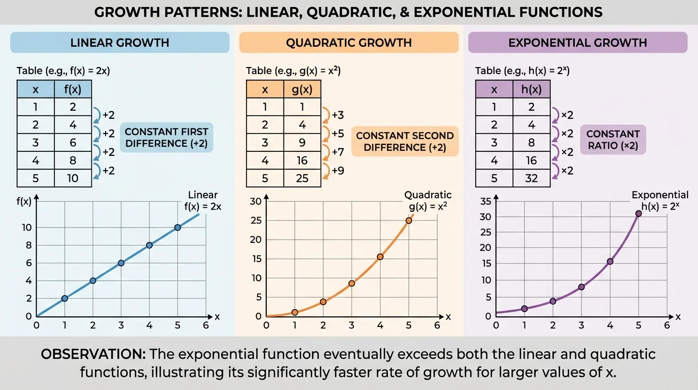
To compare them clearly, we often use three tools: equations, tables, and graphs. As [Figure 1] shows, equations show the rule. Tables reveal numerical patterns. Graphs show the long-term behavior in a visual way.
Linear function: a function that changes by a constant amount for equal changes in the input, often written as \(y = mx + b\).
Quadratic function: a function whose highest power of the variable is \(x^2\), often written as \(y = ax^2 + bx + c\).
Exponential function: a function in which the variable is in the exponent, often written as \(y = ab^x\) with \(a \ne 0\), \(b > 0\), and \(b \ne 1\).
Polynomial function: a sum of terms like \(ax^n\) where \(n\) is a whole number. Linear and quadratic functions are both polynomials.
The key question is not only how fast each function grows at first, but how its growth changes as the input becomes large.
A linear function has a constant rate of change. If a quantity grows by \(5\) each day, then after \(x\) days it can be modeled by something like \(y = 5x + 2\). The graph is a straight line, and the table has constant first differences.
A quadratic function does not grow by the same amount each time. Its first differences change, but its second differences are constant. For example, \(y = x^2\) gives values \(0, 1, 4, 9, 16\), whose first differences are \(1, 3, 5, 7\) and second differences are all \(2\).
An exponential function grows by a constant factor or ratio. For example, \(y = 2^x\) gives \(1, 2, 4, 8, 16\). Each value is multiplied by \(2\) to get the next. This repeated multiplication is what eventually makes exponential growth so powerful.
Why multiplication beats addition in the long run
If you add the same amount repeatedly, growth stays steady. If you multiply repeatedly, the amount being added gets larger and larger because each increase is based on a bigger current value. That is why \(2^x\) starts modestly but eventually rises much faster than \(10x\) or even \(x^2\).
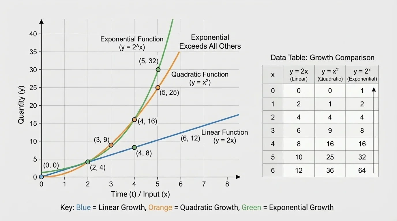
As [Figure 2] suggests, you can think of it this way: linear growth keeps taking equal steps, quadratic growth takes larger and larger steps in a patterned way, and exponential growth keeps increasing the size of its own steps.
Tables are often the fastest way to recognize what kind of growth you are seeing. Linear data has a constant first difference, quadratic data has a constant second difference, and exponential data has a constant ratio between consecutive outputs.
Consider these three functions: \(y = 3x + 1\), \(y = x^2\), and \(y = 2^x\).
| \(x\) | \(3x + 1\) | \(x^2\) | \(2^x\) |
|---|---|---|---|
| \(0\) | \(1\) | \(0\) | \(1\) |
| \(1\) | \(4\) | \(1\) | \(2\) |
| \(2\) | \(7\) | \(4\) | \(4\) |
| \(3\) | \(10\) | \(9\) | \(8\) |
| \(4\) | \(13\) | \(16\) | \(16\) |
| \(5\) | \(16\) | \(25\) | \(32\) |
Table 1. Values of a linear, quadratic, and exponential function for the same inputs.
At first, the quadratic function is larger than the exponential one for some values. At \(x = 3\), we have \(x^2 = 9\) while \(2^x = 8\). But by \(x = 5\), the exponential value is \(32\), which is already greater than \(25\). This is the kind of "eventually" statement that matters.
Tables also help you avoid a common mistake: assuming the biggest early values will stay biggest forever. That is often false when exponential growth is involved.
The graph makes the long-term story even clearer. On the same coordinate plane, a line rises steadily, a parabola curves upward, and an exponential graph begins slowly but eventually turns sharply upward and crosses above the others.
For example, compare \(y = 2x + 3\), \(y = x^2\), and \(y = 2^x\). Near the left side of the graph, the line or the parabola may be above the exponential curve. But as \(x\) increases, the exponential graph becomes steeper and steeper. It does not just continue upward; it accelerates upward.
Graphically, when one function exceeds another, that means its graph lies above the other graph. If the exponential graph crosses a line and never comes back below it for larger \(x\)-values, then the exponential function has eventually exceeded the linear function.
This does not mean exponential functions are always bigger for every input. "Eventually exceeds" means that beyond some value of \(x\), the exponential output is greater than the other output and stays greater for all larger \(x\).
Let us compare \(f(x) = 5x\) and \(g(x) = 2^x\) and determine when the exponential function exceeds the linear one.
Worked example
Step 1: Make a table of values.
| \(x\) | \(5x\) | \(2^x\) |
|---|---|---|
| \(1\) | \(5\) | \(2\) |
| \(2\) | \(10\) | \(4\) |
| \(3\) | \(15\) | \(8\) |
| \(4\) | \(20\) | \(16\) |
| \(5\) | \(25\) | \(32\) |
Table 2. Comparison of the linear function \(5x\) and the exponential function \(2^x\).
Step 2: Compare the outputs.
For \(x = 1, 2, 3, 4\), the linear function is larger. At \(x = 5\), the exponential function becomes larger because \(2^5 = 32\) and \(5 \cdot 5 = 25\).
Step 3: Check what happens after that.
At \(x = 6\), \(2^6 = 64\) and \(5(6) = 30\). The gap gets bigger. At \(x = 10\), \(2^{10} = 1024\) and \(5(10) = 50\).
So \(g(x) = 2^x\) exceeds \(f(x) = 5x\) starting at \(x = 5\), and the difference keeps increasing.
This example is powerful because the line starts off ahead. If you looked only at \(x = 1, 2, 3, 4\), you might guess the line would stay larger. The table proves otherwise.
Now compare \(f(x) = x^2\) and \(g(x) = 2^x\).
Worked example
Step 1: Evaluate both functions for several values of \(x\).
For \(x = 2\), \(x^2 = 4\) and \(2^x = 4\).
For \(x = 3\), \(x^2 = 9\) and \(2^x = 8\).
For \(x = 4\), \(x^2 = 16\) and \(2^x = 16\).
For \(x = 5\), \(x^2 = 25\) and \(2^x = 32\).
Step 2: Identify when the exponential becomes larger.
The two functions are equal at \(x = 2\) and \(x = 4\). The quadratic is larger at \(x = 3\), but the exponential is larger at \(x = 5\).
Step 3: Test larger values.
At \(x = 8\), \(x^2 = 64\) but \(2^x = 256\). At \(x = 10\), \(x^2 = 100\) while \(2^{10} = 1024\).
The exponential function eventually exceeds the quadratic function, and then grows much faster.
This is one of the most important visual ideas: a parabola curves upward, but an exponential graph turns upward more dramatically and dominates for large inputs.
Students sometimes think that using a bigger coefficient will permanently defeat exponential growth. Let us test \(f(x) = 100x^2\) and \(g(x) = 3^x\).
Worked example
Step 1: Compare a few early values.
At \(x = 2\), \(100x^2 = 400\) and \(3^x = 9\).
At \(x = 4\), \(100x^2 = 1600\) and \(3^x = 81\).
At \(x = 6\), \(100x^2 = 3600\) and \(3^x = 729\).
Step 2: Jump to larger values.
At \(x = 10\), \(100x^2 = 10,000\) and \(3^{10} = 59,049\).
Step 3: Interpret the result.
Even though the quadratic starts far larger, the exponential catches up and passes it. Once that happens, the exponential pulls away quickly.
A large coefficient may delay the crossover point, but it does not prevent it.
This is why the word eventually matters. Exponential growth may not win right away, but if the base is greater than \(1\), it wins in the long run against polynomial growth.
A polynomial function can have degree \(1\), \(2\), \(3\), or higher, such as \(7x^5 - 2x^3 + 9\). Higher-degree polynomials can grow very quickly, but their growth is still based on powers of \(x\). Exponential functions grow by repeatedly multiplying by a constant factor, such as \(2\) or \(1.05\).
The general principle is: if \(b > 1\), then \(b^x\) eventually exceeds any polynomial \(p(x)\) for sufficiently large \(x\). You do not need advanced calculus to observe this in graphs and tables. Compute enough values, and the exponential term will eventually dominate.
For instance, compare \(x^5\) and \(2^x\). For moderate values such as \(x = 10\), the polynomial is larger because \(10^5 = 100,000\) while \(2^{10} = 1024\). But later, exponential growth overtakes it. At \(x = 20\), \(x^5 = 3,200,000\) and \(2^{20} = 1,048,576\), so the polynomial is still ahead. Yet by \(x = 30\), \(x^5 = 24,300,000\) while \(2^{30} = 1,073,741,824\). The exponential has now passed it by a huge amount.
The phrase eventually exceeds is not just classroom language. It is a precise statement about long-term behavior: there exists some value of \(x\) after which one function is always greater than the other.
This idea is one reason exponential models are so important in science, economics, and technology. Human intuition is often poor at judging repeated multiplication.
One common misconception is that a larger starting value guarantees long-term dominance. Not true. A function like \(y = 1,000x\) starts much larger than \(y = 2^x\) for many values of \(x\), but the exponential function still eventually exceeds it.
Another misconception is that "increasing exponentially" means "increasing very fast immediately." Actually, exponential growth can begin slowly. If the base is close to \(1\), such as \(1.03^x\), the increase may look small at first. But over enough time, repeated percentage growth becomes significant.
It is also important to pay attention to the domain. Many real-world models only make sense for \(x \ge 0\), where \(x\) may represent time. In that setting, we compare the functions over nonnegative values of \(x\).
When reading a table, look for patterns. Constant first difference suggests linear growth. Constant second difference suggests quadratic growth. Constant ratio suggests exponential growth.
If the exponential function is decreasing, such as \(y = \left(\dfrac{1}{2}\right)^x\), then it will not exceed increasing polynomial functions for large positive \(x\). The statement in this lesson applies to increasing exponential functions, where the base satisfies \(b > 1\).
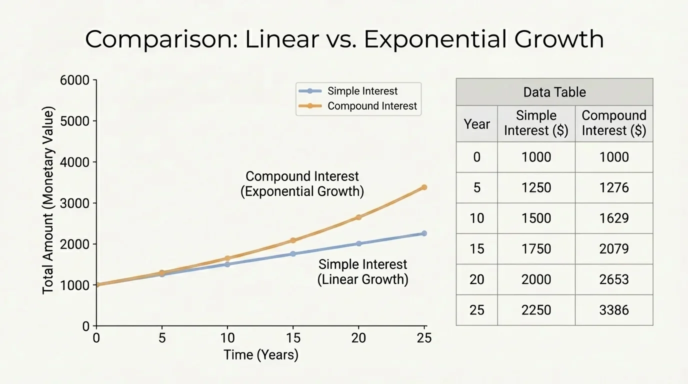
Money offers a classic comparison. A simple-interest account grows linearly because it adds the same amount each year. A compound-interest account grows exponentially because each year's interest is earned on a larger balance than the year before. The two models may begin close together, but over time the compound-interest curve rises above the simple-interest line.
As [Figure 3] shows, suppose \(\$1,000\) is invested at \(10\%\) annual interest. With simple interest, the amount after \(t\) years is \(A = 1000 + 100t\). With compound growth, the amount is \(A = 1000(1.1)^t\). At first, the amounts may seem similar. But after enough years, the exponential model becomes much larger.
Population growth can also be exponential when each generation is larger by a percentage rather than by a fixed number. Technology provides another example: if computing capacity doubles regularly, the resulting pattern is exponential, not linear. That helps explain why some technological changes appear slow for years and then suddenly seem to explode.
In epidemiology, the early spread of a disease can follow exponential growth when each infected person infects multiple others. This is one reason small early increases can become serious quickly. The pattern echoes what we saw in [Figure 1]: repeated multiplication creates outputs that eventually surge past additive models.
These applications all share the same mathematical structure. The details differ, but the long-term comparison remains: growth by repeated multiplication eventually exceeds growth by repeated addition or by powers of the input.
When you are given a table or graph and asked to compare growth, use a clear strategy.
First, look at the table. If the outputs change by a constant amount, the model is linear. If the first differences are not constant but the second differences are, the model is quadratic. If consecutive outputs have a constant ratio, the model is exponential.
Second, look at the graph. A straight line suggests linear growth. A U-shaped curve suggests quadratic behavior. A curve that rises slowly and then sharply upward suggests exponential growth.
Third, think long-term. Do not stop after the first few values. Extend the table or imagine moving farther to the right on the graph. The question is about what happens eventually, not just what happens first.
"The most dangerous phrase in comparing growth is: 'It has always been smaller so it will stay smaller.'"
That statement is not a formal theorem, but it captures an important habit of mind. In function analysis, long-term behavior matters.