When engineers design a bridge or when data scientists fit curves to data, they pay close attention to the points where those curves hit the horizontal axis. These special points are called zeros of the function, and for polynomials, they are often the key to understanding the whole graph 🧮.
Every polynomial function models some kind of relationship: position over time, profit over number of items, intensity over distance, and so on. The zeros of the function are the inputs where the output is zero. On a graph of a function, these show up as x-intercepts, where the graph crosses or just touches the horizontal axis.
For example, if a function describes the height of a ball over time, its zeros tell you when the ball is on the ground. If a function describes profit, its zeros tell you the break-even points. Understanding how to find these zeros quickly and then sketch a rough graph gives you powerful insight into many real situations.
Polynomial is an expression like \(2x^3 - 5x^2 + x - 3\) made by adding and subtracting terms of the form \(ax^n\), where \(a\) is a real number and \(n\) is a nonnegative integer.
Factor of a polynomial is an expression, such as \((x - 2)\), that multiplies with other expressions to give the polynomial, for example \((x - 2)(x + 3) = x^2 + x - 6\).
Zero (or root) of a polynomial function is a number \(r\) such that the function value is zero: \(f(r) = 0\).
x-intercept of a graph is a point where the graph meets the horizontal axis, so its coordinates are \((r, 0)\).
These ideas are tied together by one crucial algebra property that you may already know.
The connection between zeros and factors comes from the zero-product property: if a product of numbers is zero, then at least one factor must be zero. In symbols, if \(AB = 0\), then \(A = 0\) or \(B = 0\) (or both).
Now suppose we factor a polynomial function like \(f(x) = (x - 2)(x + 3)\). To find its zeros, we solve \(f(x) = 0\):
\[(x - 2)(x + 3) = 0\]
By the zero-product property, this equation is true exactly when either \(x - 2 = 0\) or \(x + 3 = 0\). So the solutions are \(x = 2\) and \(x = -3\). These are the zeros of the function and the x-intercepts of its graph.
This leads to a powerful rule:
Relationship between factors and zeros of polynomials
If a polynomial function \(f(x)\) has a factor \((x - r)\), then \(x = r\) is a zero of the function, and the point \((r, 0)\) is an x-intercept of the graph. Conversely, if \(r\) is a zero of a polynomial, then \((x - r)\) is a factor of that polynomial.
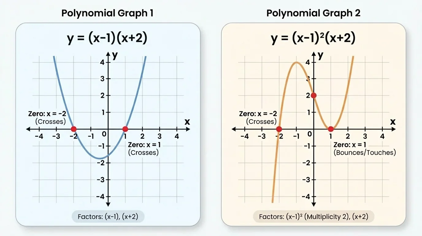
Sometimes a factor shows up more than once. For example, \(f(x) = (x - 1)^2(x + 4)\). The factor \((x - 1)\) has multiplicity 2, and \((x + 4)\) has multiplicity 1. This affects how the graph behaves at the corresponding x-intercepts.
Assume you already have a polynomial written in factored form, such as \(f(x) = a(x - r_1)(x - r_2)\cdots(x - r_n)\), where \(a\) is a nonzero constant. Then finding the zeros is straightforward:
Here is a quick reference:
| Factor | Zero | Multiplicity |
|---|---|---|
| \((x - 5)\) | \(x = 5\) | 1 |
| \((x + 2)\) | \(x = -2\) | 1 |
| \((2x - 3)\) | \(x = \dfrac{3}{2}\) | 1 |
| \((x - 1)^3\) | \(x = 1\) | 3 |
Important: Nonzero constant factors like \(2\), \(-5\), or \(\dfrac{1}{2}\) never create or remove zeros. Only the factors that contain \(x\) matter for locating zeros.
Often, a polynomial is not given to you in factored form. To use the connection between factors and zeros, you first need to factor it. Some common factoring techniques you should recall:
Once the polynomial is factored, you are ready to find its zeros and then think about the graph.
A polynomial function \(f(x)\) can be graphed on a coordinate plane. The graph is a smooth, continuous curve (no jumps or holes). The end behavior of the graph is determined by the leading term (the term with highest degree), and the x-intercepts are determined by the zeros. Together, these features let you draw a good rough sketch.
The graphs in [Figure 1] highlight how zeros appear as x-intercepts and how multiplicity changes the graph's behavior at those points.
Degree and end behavior
Multiplicity and local behavior at zeros
In addition, a polynomial of degree \(n\) has at most \(n - 1\) turning points (local maxima and minima). This helps you imagine how the curve wiggles between its intercepts.
Graph behavior near zeros and at infinity
Near each zero with odd multiplicity, the graph passes through the x-axis, changing sign from positive to negative or vice versa. Near each zero with even multiplicity, the graph touches the x-axis and turns back the way it came, staying on the same side of the axis. Far left and far right, the graph follows the direction of the leading term, like \(x^3\), \(-x^3\), \(x^4\), and so on.
Putting these pieces together lets you sketch accurate rough graphs even without a calculator 🙂.
Example 1: Quadratic with two distinct zeros
Let \(f(x) = x^2 - x - 6\). Find the zeros and sketch a rough graph.
Step 1: Factor the polynomial
We need two numbers that multiply to \(-6\) and add to \(-1\). These are \(-3\) and \(2\). So
\[x^2 - x - 6 = (x - 3)(x + 2).\]
Step 2: Use factors to find zeros
Set each factor equal to zero:
\[x - 3 = 0 \Rightarrow x = 3,\]
\[x + 2 = 0 \Rightarrow x = -2.\]
So the zeros of \(f(x)\) are \(x = -2\) and \(x = 3\). The x-intercepts are \((-2, 0)\) and \((3, 0)\).
Step 3: Use degree and leading coefficient
The polynomial is degree 2 with leading coefficient \(1\) (positive). So both ends of the graph go up. It is a parabola opening upward.
Step 4: Sketch the rough graph
Plot the intercepts at \((-2, 0)\) and \((3, 0)\). Draw a U-shaped curve opening up that crosses the x-axis at those points. You might also find the vertex, but for a rough sketch, the intercepts and end behavior are the key.
The zeros are \(x = -2\) and \(x = 3\).
Notice how easily the zeros came from the factors.
Example 2: Quadratic with a repeated zero
Let \(g(x) = (x + 1)^2\). Find the zeros and describe the graph's behavior at the intercept.
Step 1: Identify the factor and multiplicity
The polynomial is already factored: \(g(x) = (x + 1)^2\). The factor \((x + 1)\) has multiplicity 2 (an even multiplicity).
Step 2: Find the zero
Set \(x + 1 = 0\):
\(x = -1.\)
There is a single zero at \(x = -1\), with multiplicity 2. The x-intercept is \((-1, 0)\).
Step 3: Describe the shape
This is a degree 2 polynomial with positive leading coefficient (it is just a shifted version of \(x^2\)), so it opens upward. Because the zero at \(x = -1\) has even multiplicity, the graph touches the x-axis at \((-1, 0)\) and turns around there instead of crossing through.
So the graph is a parabola opening up with its lowest point on the x-axis at \((-1, 0)\).
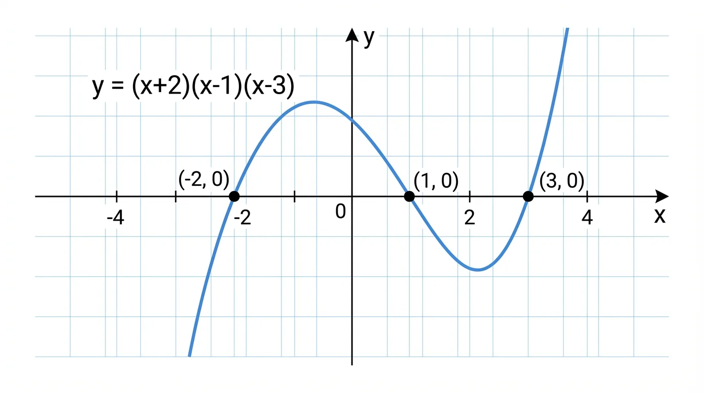
Example 3: Cubic with three real zeros
Consider \(h(x) = (x + 2)(x - 1)(x - 3)\). Find all zeros and sketch a rough graph, noting how many times the graph can turn. The final sketch is shown in [Figure 2].
Step 1: Read zeros from factors
Each linear factor gives one zero:
\[x + 2 = 0 \Rightarrow x = -2,\]
\[x - 1 = 0 \Rightarrow x = 1,\]
\[x - 3 = 0 \Rightarrow x = 3.\]
All multiplicities are 1 (odd), so the graph will cross the x-axis at each of these points.
Step 2: Determine degree and leading coefficient
Multiplying the leading \(x\)-terms from each factor gives \(x \cdot x \cdot x = x^3\), so this is a degree 3 polynomial with positive leading coefficient.
Thus the end behavior is: as \(x \to -\infty\), \(h(x) \to -\infty\), and as \(x \to +\infty\), \(h(x) \to +\infty\).
Step 3: Use turning point information
A cubic (degree 3) polynomial can have at most \(3 - 1 = 2\) turning points. So the graph will wiggle at most twice as it passes through the three intercepts.
Step 4: Sketch the rough graph
Plot the x-intercepts at \((-2, 0)\), \((1, 0)\), and \((3, 0)\). Draw the left end coming from below, crossing the x-axis at \(-2\), then rising to a local maximum, crossing again at \(1\), dipping to a local minimum, crossing at \(3\), and finally rising to the right.
The graph passes through all three intercepts and shows two turning points, as the cubic in [Figure 2] illustrates.
Example 4: Polynomial with complex zeros (not visible as x-intercepts)
Let \(p(x) = (x - 4)(x^2 + 1)\). Find the real zeros and explain what appears on the graph.
Step 1: Solve each factor
From \(x - 4 = 0\), we get \(x = 4\), a real zero.
From \(x^2 + 1 = 0\), we get \(x^2 = -1\), so \(x = \pm i\), which are not real numbers.
Step 2: Interpret the graph
On a standard coordinate plane with a real x-axis and y-axis, only real zeros appear as x-intercepts. So the graph of \(p(x)\) has a single x-intercept at \((4, 0)\). The other two (complex) zeros do not show up as x-intercepts but still influence the overall shape.
Recognizing that not every zero must be real is important when interpreting polynomial graphs.
Polynomial models appear in many real-world situations, and their zeros often mark important events or thresholds 🌍.
In physics, the height \(h(t)\) of a thrown object over time \(t\) can often be modeled by a quadratic polynomial such as \(h(t) = -5t^2 + 20t\). The zeros of \(h(t)\) tell you when the object is at ground level. The graph in [Figure 3] shows this idea.
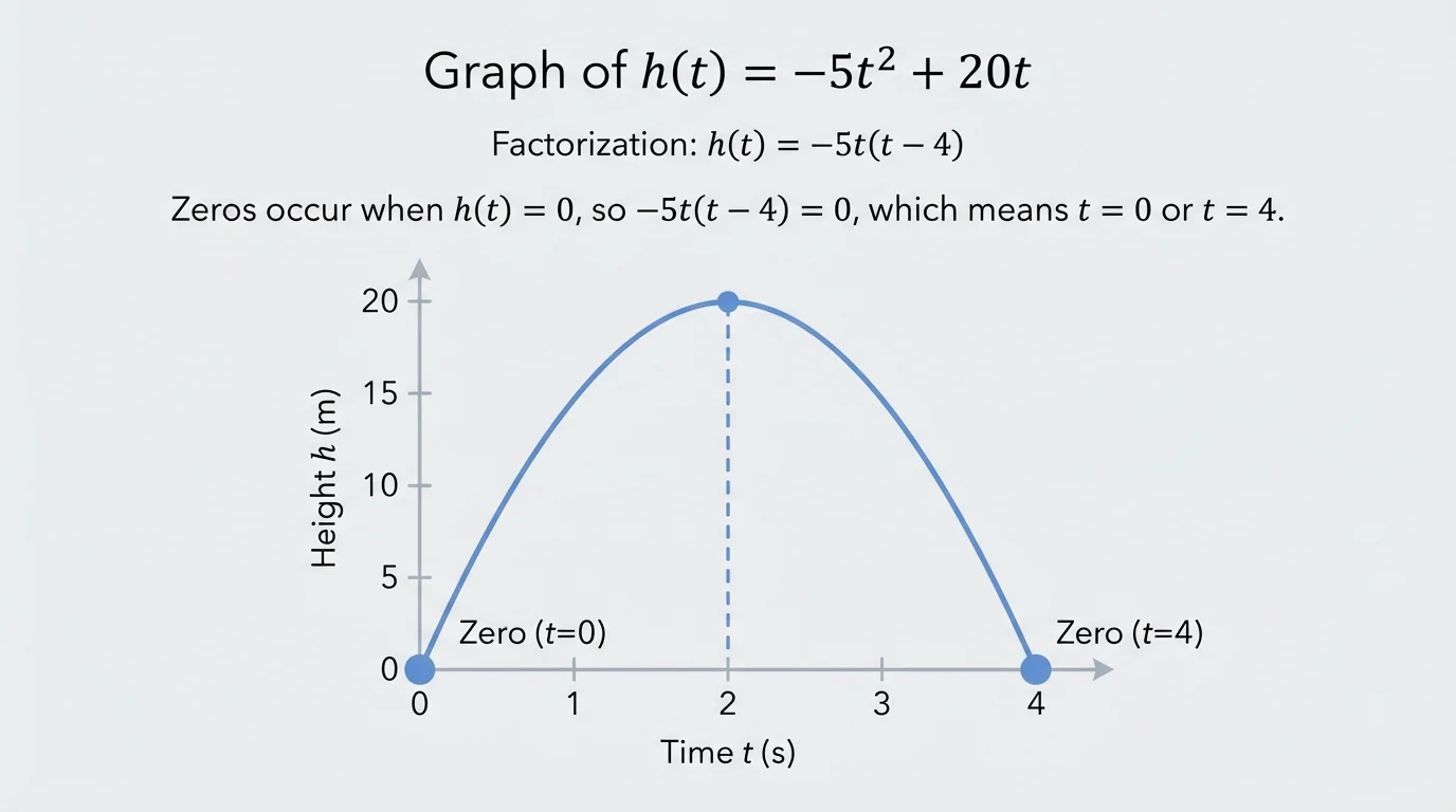
For \(h(t) = -5t^2 + 20t\), factoring gives:
\[-5t^2 + 20t = -5t(t - 4).\]
The zeros are \(t = 0\) and \(t = 4\). Interpreting these, the object is on the ground at time 0 (when it is thrown) and again at time 4 (when it lands). Between these times, the graph is above the axis, representing positive height.
In business, a polynomial may approximate profit \(P(x)\) based on the number of units sold, \(x\). Zeros of \(P(x)\) tell you the break-even points where profit is zero. Between those points, the sign of \(P(x)\) indicates profit (positive) or loss (negative).
In computer graphics, curves used to design fonts and smooth shapes (such as Bézier curves) can be expressed using polynomials. Zeros can mark where parts of the curve intersect axes or other reference lines, which matters in layout and animation.
Polynomial equations are central in control systems for airplanes and rockets, where the roots of certain polynomials determine whether the system is stable or will start to oscillate uncontrollably.
In all these situations, understanding where the polynomial is zero helps you understand when something starts, ends, hits a boundary, or changes behavior.
When working with zeros and graphs of polynomials, certain errors show up over and over. Being aware of them helps you avoid traps.
By combining accurate factoring, careful use of the zero-product property, and attention to degree, leading coefficient, and multiplicities, you can confidently move from a polynomial formula to a meaningful rough sketch of its graph 🎯.