Every day, people make decisions under limits: a business has limited materials, an athlete has limited training time, and a family has a limited budget. Algebra becomes especially powerful when it helps answer a simple but serious question: Which choices are actually possible? That is what constraints are about. A model may suggest many combinations, but only some satisfy all the rules of the situation. In mathematics, we represent those rules with equations, inequalities, or systems, and then interpret the solutions as options that work or options that do not.
A constraint is a condition that limits what values a variable can take. If a school club has at most $200 to spend, then the total cost must stay less than or equal to $200. If a nutrition plan requires at least \(50\) grams of protein, then the protein amount must be greater than or equal to \(50\).
An equation models an exact relationship, such as a total or a balance, where two expressions are equal.
An inequality models a range of possible values, such as being less than, greater than, at most, or at least a certain amount.
A system is a set of equations and/or inequalities that must all be true at the same time.
A viable solution is a value or ordered pair that satisfies every condition in the context. A nonviable solution fails at least one condition.
In modeling, the variables usually stand for quantities in a real situation. For example, \(x\) might be the number of sandwiches and \(y\) the number of salads. A point such as \((4, 3)\) then means \(4\) sandwiches and \(3\) salads. The key question is not just whether \((4, 3)\) is on a graph, but whether it makes sense and satisfies the real-world limits.
Some constraints are expressed by equations because the relationship must be exact. For instance, if a total of \(120\) tickets were sold, then the numbers of student and adult tickets must satisfy \(s + a = 120\). Other constraints are expressed by inequalities because many values are possible. If the revenue must be at least $700, then the model might be \(5s + 8a \ge 700\).
To build a model, start by choosing variables clearly. Then translate each condition one at a time. This works best when you ask: What quantity is being limited, and in which direction?
Common phrases translate in predictable ways:
| Words in context | Mathematical meaning |
|---|---|
| at most | \(\le\) |
| no more than | \(\le\) |
| at least | \(\ge\) |
| no fewer than | \(\ge\) |
| exactly | \(=\) |
| less than | \(<\) |
| greater than | \(>\) |
Table 1. Common verbal phrases and the mathematical symbols they usually represent.
Suppose a streaming startup offers two plans: basic and premium. Let \(b\) be the number of basic subscriptions and \(p\) the number of premium subscriptions. If server capacity allows no more than \(1{,}000\) users, then \(b + p \le 1{,}000\). If the company wants at least \(300\) premium subscriptions, then \(p \ge 300\). If each basic plan brings in $8 and each premium plan brings in $12, and the goal is exactly $10,000 in revenue, then \(8b + 12p = 10{,}000\).
When you write an expression like \(8b + 12p\), you are combining coefficients and variables to represent a total. The coefficient tells how much one unit of the variable contributes. Here, each basic plan adds \(8\) and each premium plan adds \(12\).
Notice that one situation can involve both equations and inequalities. That is normal in modeling. Real situations often have one exact condition, several limits, and sometimes additional restrictions such as \(b \ge 0\) and \(p \ge 0\), because negative subscriptions do not make sense.
A system of inequalities or system of equations is used when several conditions must hold at once. Each equation or inequality cuts down the list of possible solutions. The final answer is the set of values that satisfy all of them together.
For example, a factory producing two products might face these conditions:
Material limit: \(2x + 3y \le 60\)
Labor limit: \(x + 2y \le 40\)
Minimum production of product \(x\): \(x \ge 10\)
Nonnegativity: \(x \ge 0\), \(y \ge 0\)
A solution such as \((12, 8)\) is viable only if it satisfies every inequality. Check:
\(2(12) + 3(8) = 24 + 24 = 48\), so \(48 \le 60\)
\(12 + 2(8) = 12 + 16 = 28\), so \(28 \le 40\)
Also, \(12 \ge 10\), \(12 \ge 0\), and \(8 \ge 0\). Therefore, \((12, 8)\) is viable.
But \((8, 15)\) is nonviable because \(2(8) + 3(15) = 16 + 45 = 61\), and \(61 > 60\), so it breaks the material limit. It also fails the condition \(x \ge 10\).
When two variables are involved, graphing often makes the situation much easier to understand. The overlap of all the allowed regions forms the set of possible solutions, as [Figure 1] shows. This overlap is often called the feasible region.
Why the feasible region matters
Each inequality represents a half-plane: one side of a boundary line. The solutions to the full system are found where all the correct half-planes overlap. Any point inside or on the boundary of that overlap is viable, as long as the context allows it.
If the inequality is \(y \le 2x + 3\), first graph the boundary line \(y = 2x + 3\). Because the symbol is \(\le\), the boundary is included, so the line is solid. Then shade the region below the line. If the inequality were \(y > 2x + 3\), the boundary line would be dashed, and the region above it would be shaded.
In many modeling situations, the variables count things, so the first quadrant is the important part of the graph because \(x \ge 0\) and \(y \ge 0\). This keeps attention on the first quadrant and on the overlap of constraints rather than on all possible real numbers.
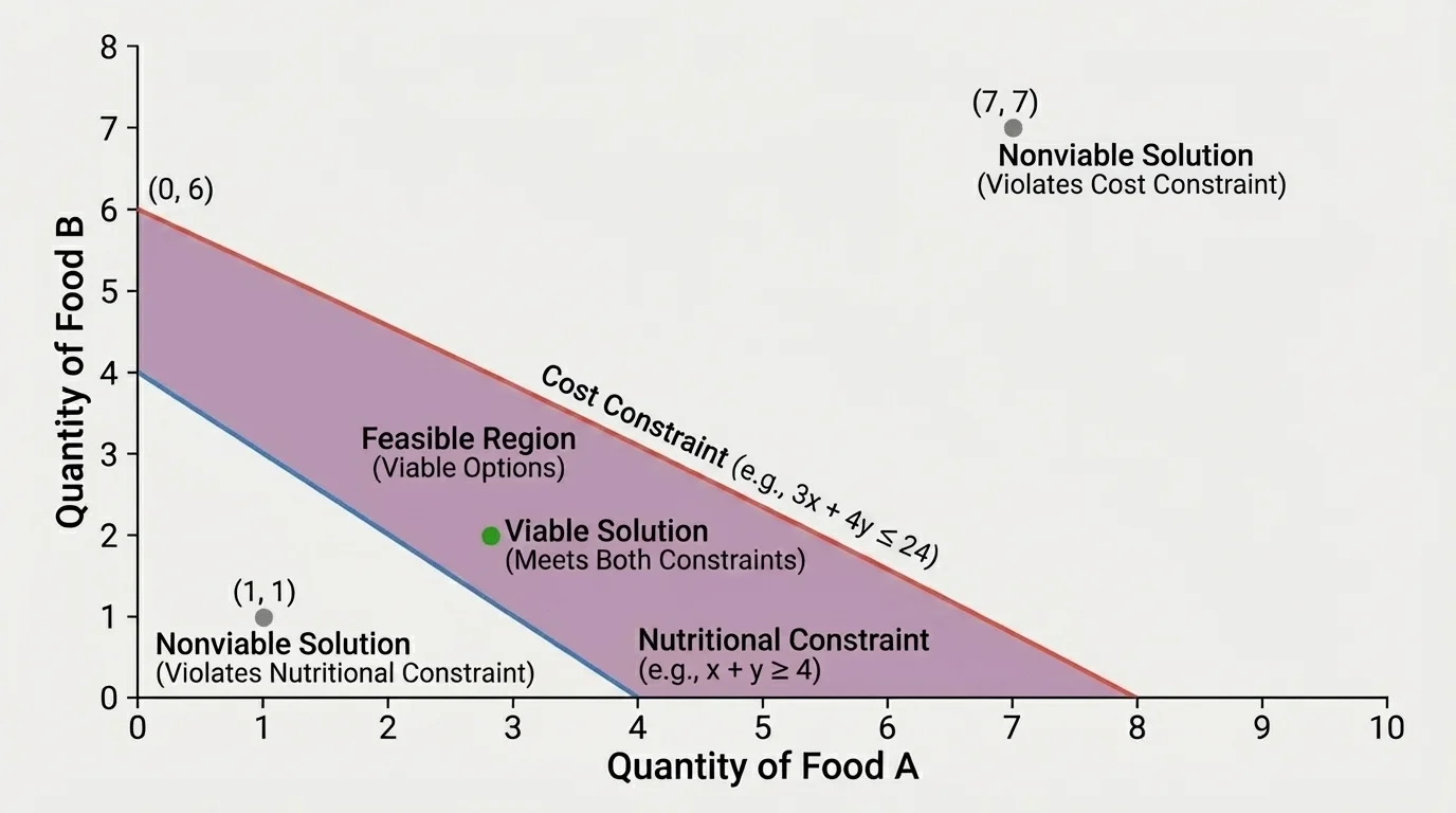
A single point on the graph represents one possible combination. If that point lies inside the feasible region, it is viable. If it lies outside, it is nonviable. Boundary points also matter. For example, if a budget condition is \(3x + 2y \le 18\), then any point on the line \(3x + 2y = 18\) uses the entire budget exactly.
Sometimes the graph includes only integer points that make sense. If \(x\) is the number of buses and \(y\) is the number of vans, then \((2.5, 4)\) may satisfy the algebra, but it is not a viable real-world option because half a bus is impossible. This is one reason context always matters.
In business and engineering, large decision problems with many variables are often solved by optimization methods built on the same idea: define constraints, find the feasible region, and then search for the best viable solution.
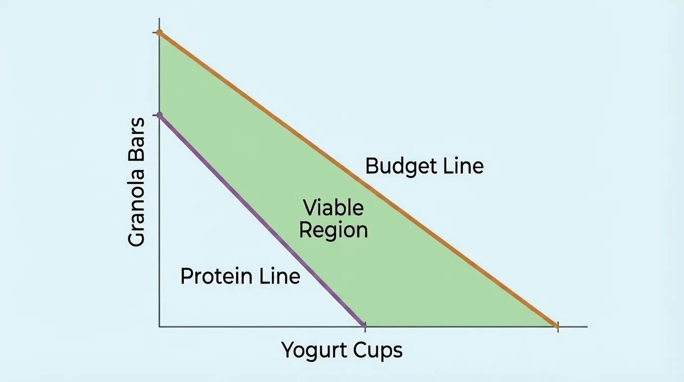
A school cafeteria wants to design a simple meal using two foods: yogurt cups and granola bars. Let \(x\) be the number of yogurt cups and \(y\) the number of granola bars. Each yogurt cup costs $1.50 and provides \(8\) grams of protein. Each granola bar costs $2.00 and provides \(5\) grams of protein. The meal must cost no more than $12.00 and provide at least \(35\) grams of protein. Also, \(x \ge 0\) and \(y \ge 0\). This situation can be represented on a graph, as [Figure 2] shows, because each pair \((x, y)\) represents one possible meal combination.
Worked example: writing and checking the system
Step 1: Write the cost constraint.
Each yogurt cup costs $1.50 and each granola bar costs $2.00, so the total cost is \(1.5x + 2y\).
The meal costs no more than $12.00, so:
\[1.5x + 2y \le 12\]
Step 2: Write the protein constraint.
Each yogurt cup gives \(8\) grams of protein and each granola bar gives \(5\) grams. The total protein is \(8x + 5y\).
The meal must provide at least \(35\) grams, so:
\[8x + 5y \ge 35\]
Step 3: Include nonnegativity constraints.
Numbers of food items cannot be negative:
\[x \ge 0, \quad y \ge 0\]
Step 4: Test a possible solution.
Try \((x, y) = (3, 3)\).
Cost: \(1.5(3) + 2(3) = 4.5 + 6 = 10.5\), and \(10.5 \le 12\)
Protein: \(8(3) + 5(3) = 24 + 15 = 39\), and \(39 \ge 35\)
So \((3, 3)\) is viable.
Step 5: Test a nonviable solution.
Try \((1, 4)\).
Cost: \(1.5(1) + 2(4) = 1.5 + 8 = 9.5\), so the cost works.
Protein: \(8(1) + 5(4) = 8 + 20 = 28\), and \(28 < 35\)
So \((1, 4)\) is nonviable because it fails the protein requirement.
To graph the system, use the boundary lines \(1.5x + 2y = 12\) and \(8x + 5y = 35\). The first inequality shades below the cost line, while the second shades above the protein line. The overlap in the first quadrant gives the viable meal combinations.
In a real cafeteria, whole items are usually required, so integer points such as \((2, 4)\) or \((4, 2)\) are more realistic than fractional points. A point may lie in the feasible region algebraically but still need interpretation based on whether partial items are allowed.
A theater sold a total of \(150\) tickets for one show. Student tickets cost $6 and adult tickets cost $10. The theater earned at least $1,200. Let \(s\) be the number of student tickets and \(a\) be the number of adult tickets.
Worked example: equation plus inequality
Step 1: Write the total-ticket equation.
The total number of tickets is exactly \(150\), so:
\(s + a = 150\)
Step 2: Write the revenue inequality.
Revenue is \(6s + 10a\). Since the theater earned at least $1,200:
\[6s + 10a \ge 1200\]
Step 3: Use substitution to interpret the condition.
From \(s + a = 150\), we get \(s = 150 - a\).
Substitute into the revenue inequality:
\(6(150 - a) + 10a \ge 1200\)
\(900 - 6a + 10a \ge 1200\)
\(900 + 4a \ge 1200\)
\(4a \ge 300\)
\(a \ge 75\)
Step 4: Interpret the result.
The number of adult tickets must be at least \(75\). Since \(s + a = 150\), this also means student tickets must be at most \(75\).
This example shows that a system can combine an exact total with a lower bound. Every solution on the line \(s + a = 150\) represents exactly \(150\) tickets, but only the part of that line satisfying \(6s + 10a \ge 1200\) is viable.
If someone claims \((90, 60)\) is a solution, check both conditions. First, \(90 + 60 = 150\), so the total works. Revenue is \(6(90) + 10(60) = 540 + 600 = 1{,}140\). Since \(1{,}140 < 1{,}200\), it is nonviable.
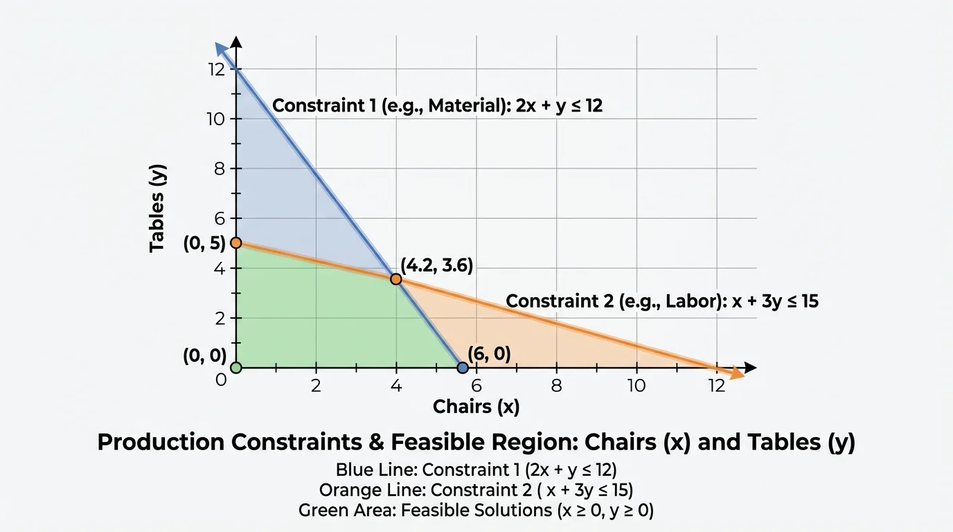
A furniture shop makes chairs and tables. Let \(c\) be the number of chairs and \(t\) the number of tables. Each chair requires \(2\) hours of carpentry and \(1\) hour of finishing. Each table requires \(4\) hours of carpentry and \(3\) hours of finishing. The shop has at most \(40\) carpentry hours and at most \(24\) finishing hours available. The feasible polygon on the graph, as [Figure 3] shows, represents every production plan that fits both time limits.
Worked example: system and feasible region
Step 1: Write the carpentry constraint.
Chairs use \(2\) hours each and tables use \(4\) hours each:
\[2c + 4t \le 40\]
Step 2: Write the finishing constraint.
Chairs use \(1\) hour each and tables use \(3\) hours each:
\[c + 3t \le 24\]
Step 3: Include nonnegativity.
\[c \ge 0, \quad t \ge 0\]
Step 4: Test a point.
Try \((c, t) = (8, 5)\).
Carpentry: \(2(8) + 4(5) = 16 + 20 = 36\), and \(36 \le 40\)
Finishing: \(8 + 3(5) = 8 + 15 = 23\), and \(23 \le 24\)
So \((8, 5)\) is viable.
Step 5: Test a nonviable point.
Try \((10, 6)\).
Carpentry: \(2(10) + 4(6) = 20 + 24 = 44\), and \(44 > 40\)
So \((10, 6)\) is nonviable.
To understand the boundaries better, simplify the carpentry equation \(2c + 4t = 40\) to \(c + 2t = 20\). The intercepts are \((20, 0)\) and \((0, 10)\). For the finishing equation \(c + 3t = 24\), the intercepts are \((24, 0)\) and \((0, 8)\). These lines bound the region of possible plans.
This graph makes an important modeling idea visible: the intersection of constraints forms a polygonal region, and every point inside it is a workable plan. In more advanced optimization problems, the best profit often occurs at a corner point of this region.
One common mistake is reversing an inequality symbol. If a problem says "at least \(20\)," the correct symbol is \(\ge\), not \(\le\). If it says "no more than \(50\)," the correct symbol is \(\le\).
Another mistake is forgetting nonnegativity constraints. In many models, \(x \ge 0\) and \(y \ge 0\) are necessary because negative items, hours, or people are impossible.
A third mistake is treating every algebraic solution as meaningful. Suppose a system gives \((2.7, 4.4)\). If the variables represent liters of a liquid, that may be fine. If they represent buses and drivers, it is not.
Discrete versus continuous solutions
Some contexts allow any real number in a range, such as time, mass, or distance. These are continuous solutions. Other contexts involve counting whole objects, such as tickets, meals, or machines. These are often discrete solutions, so only integer values are viable even if the graph shows a full shaded region.
Boundary lines also need careful interpretation. If the inequality is \(\le\) or \(\ge\), the boundary counts as part of the solution set. If the inequality is \(<\) or \(>\), the boundary is excluded. This difference can matter in contexts such as safety limits, legal limits, or exact minimum requirements.
Constraint models appear in nutrition, medicine, logistics, finance, and engineering. A hospital may balance doses of two medications under effectiveness and safety limits. A company may schedule workers under time and budget constraints. An environmental planner may choose combinations of energy sources under cost and emissions requirements.
In sports science, a training plan might limit total weekly hours while requiring minimum time in strength, endurance, and recovery activities. In economics, a household budget model can represent rent, food, transportation, and savings using equations and inequalities. In computer science, algorithms often search through possible solutions and reject nonviable options that violate constraints.
"Mathematics is not just about finding answers; it is about deciding which answers are possible."
The strongest models do more than produce numbers. They connect those numbers to decisions. When you build equations and inequalities from a context, you are turning real conditions into mathematical language. When you test or graph solutions, you are deciding what can actually happen.