A navigation app, a game engine, and economic forecasting can all depend on solving several equations at once. When there are many variables and many equations, guessing and checking is inefficient. Matrices turn that mess into structure, and an inverse matrix can unlock a whole system in one move.
Systems of linear equations are often first solved by graphing, substitution, or elimination. Those methods still matter, but matrices give a more compact and powerful way to organize information. They are especially useful when a system has three or more variables.
A system of equations can be written in matrix equation form, which organizes all coefficients at once, as shown in [Figure 1]. Instead of writing each equation separately, we combine the coefficients into one matrix, the variables into one column vector, and the constants into another column vector.
For example, consider the system
\[\begin{aligned}2x + 3y &= 7 \\ 5x - y &= 4\end{aligned}\]
This can be written as
\[\begin{bmatrix}2 & 3 \\ 5 & -1\end{bmatrix}\begin{bmatrix}x \\ y\end{bmatrix}=\begin{bmatrix}7 \\ 4\end{bmatrix}\]
Here, the coefficient matrix is \(A = \begin{bmatrix}2 & 3 \\ 5 & -1\end{bmatrix}\), the variable vector is \(\mathbf{x} = \begin{bmatrix}x \\ y\end{bmatrix}\), and the constant vector is \(\mathbf{b} = \begin{bmatrix}7 \\ 4\end{bmatrix}\). So the entire system becomes \(A\mathbf{x} = \mathbf{b}\).
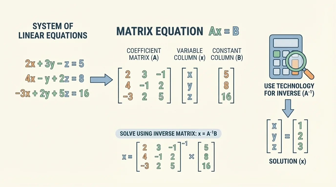
This notation matters because if \(A\) has an inverse, then we can isolate \(\mathbf{x}\) in a way that resembles solving a single-variable equation. That idea is the heart of the inverse method.
You already know that if \(ax = b\) and \(a \ne 0\), then \(x = \dfrac{b}{a}\). Matrix inverses are the matrix version of dividing by a nonzero number, but the process only works when the matrix is invertible.
Unlike ordinary numbers, matrices do not always behave the same way under multiplication. In particular, the order of multiplication matters: in general, \(AB \ne BA\). That is one reason matrix solving requires careful notation.
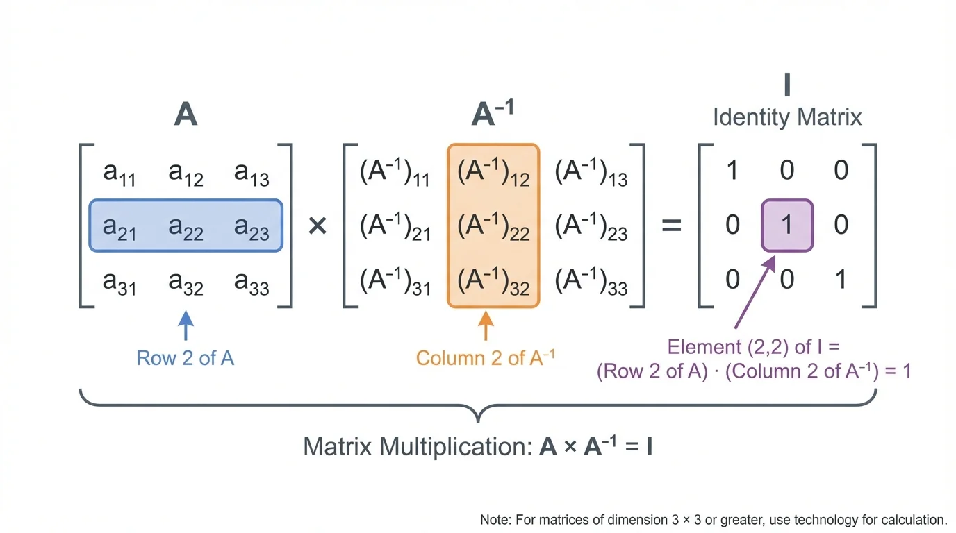
An inverse matrix plays a role similar to a reciprocal. For a nonzero number \(a\), the reciprocal is \(\dfrac{1}{a}\), because \(a \cdot \dfrac{1}{a} = 1\). For matrices, the corresponding idea is shown in [Figure 2]: if a square matrix \(A\) has an inverse, then
\[AA^{-1} = A^{-1}A = I\]
where \(I\) is the identity matrix. The identity matrix acts like the number \(1\) in matrix multiplication. For example,
\[I_2 = \begin{bmatrix}1 & 0 \\ 0 & 1\end{bmatrix}, \qquad I_3 = \begin{bmatrix}1 & 0 & 0 \\ 0 & 1 & 0 \\ 0 & 0 & 1\end{bmatrix}\]
If \(A\mathbf{x} = \mathbf{b}\) and \(A^{-1}\) exists, then multiply both sides on the left by \(A^{-1}\): \(A^{-1}(A\mathbf{x}) = A^{-1}\mathbf{b}\). Because \(A^{-1}A = I\), this becomes \(I\mathbf{x} = A^{-1}\mathbf{b}\), so \(\mathbf{x} = A^{-1}\mathbf{b}\).
Square matrix means a matrix with the same number of rows and columns.
Invertible matrix means a square matrix that has an inverse.
Singular matrix means a square matrix that does not have an inverse.
This method only applies to square matrices. A non-square matrix cannot have a two-sided inverse in this sense, so inverse methods for solving systems require the number of equations to match the number of variables.
Not every square matrix has an inverse. A key test involves the determinant. For a \(2 \times 2\) matrix
\[A = \begin{bmatrix}a & b \\ c & d\end{bmatrix}\]
the determinant is
\[\det(A) = ad - bc\]
If \(\det(A) \ne 0\), then \(A\) is invertible. If \(\det(A) = 0\), then \(A\) is singular and has no inverse.
This condition is more than a technical rule. A determinant of zero means the rows or columns do not provide enough independent information. In a system of equations, that often means the equations overlap in a dependent way or contradict each other.
A matrix can appear perfectly ordinary and still fail to have an inverse. Even a tiny change in one entry can change the determinant from nonzero to zero, which completely changes whether the system has a unique solution.
For larger matrices, the same basic idea remains true: if \(\det(A) \ne 0\), the inverse exists; if \(\det(A) = 0\), it does not.
For a \(2 \times 2\) matrix, there is a direct formula. If
\[A = \begin{bmatrix}a & b \\ c & d\end{bmatrix}\]
and \(ad - bc \ne 0\), then
\[A^{-1} = \frac{1}{ad-bc}\begin{bmatrix}d & -b \\ -c & a\end{bmatrix}\]
You can remember the pattern this way: swap the diagonal entries, change the signs of the off-diagonal entries, and divide by the determinant.
Solved example 1
Find the inverse of \(A = \begin{bmatrix}4 & 1 \\ 2 & 3\end{bmatrix}\), if it exists.
Step 1: Find the determinant.
\(\det(A) = 4 \cdot 3 - 1 \cdot 2 = 12 - 2 = 10\).
Step 2: Since \(10 \ne 0\), the inverse exists.
Step 3: Apply the inverse formula.
Swap \(4\) and \(3\), and change the signs of \(1\) and \(2\): \(\begin{bmatrix}3 & -1 \\ -2 & 4\end{bmatrix}\).
Step 4: Divide by the determinant.
\[A^{-1} = \frac{1}{10}\begin{bmatrix}3 & -1 \\ -2 & 4\end{bmatrix}\]
The inverse is \(\dfrac{1}{10}\begin{bmatrix}3 & -1 \\ -2 & 4\end{bmatrix}\).
A quick check helps: multiplying \(A\) by \(A^{-1}\) should produce the identity matrix. This verification is useful because sign errors are common when using the formula.
Once the inverse is known, solving the system becomes matrix multiplication. This is efficient when you want a method that works in a structured, repeatable way.
Solved example 2
Solve the system
\[\begin{aligned}4x + y &= 9 \\ 2x + 3y &= 13\end{aligned}\]
Step 1: Write the system as \(A\mathbf{x} = \mathbf{b}\).
\[\begin{bmatrix}4 & 1 \\ 2 & 3\end{bmatrix}\begin{bmatrix}x \\ y\end{bmatrix}=\begin{bmatrix}9 \\ 13\end{bmatrix}\]
Step 2: Use the inverse from the previous example.
\[A^{-1} = \frac{1}{10}\begin{bmatrix}3 & -1 \\ -2 & 4\end{bmatrix}\]
Step 3: Multiply both sides by \(A^{-1}\).
\(\mathbf{x} = A^{-1}\mathbf{b} = \dfrac{1}{10}\begin{bmatrix}3 & -1 \\ -2 & 4\end{bmatrix}\begin{bmatrix}9 \\ 13\end{bmatrix}\).
Step 4: Perform the matrix multiplication.
First entry: \(3 \cdot 9 + (-1) \cdot 13 = 27 - 13 = 14\).
Second entry: \((-2) \cdot 9 + 4 \cdot 13 = -18 + 52 = 34\).
So \(\mathbf{x} = \dfrac{1}{10}\begin{bmatrix}14 \\ 34\end{bmatrix} = \begin{bmatrix}\dfrac{7}{5} \\ \dfrac{17}{5}\end{bmatrix}\).
Therefore, \[x = \frac{7}{5}, \qquad y = \frac{17}{5}\]
You can verify the solution in the original system. Substituting \(x = \dfrac{7}{5}\) and \(y = \dfrac{17}{5}\) gives \(4\left(\dfrac{7}{5}\right) + \dfrac{17}{5} = \dfrac{45}{5} = 9\), and \(2\left(\dfrac{7}{5}\right) + 3\left(\dfrac{17}{5}\right) = \dfrac{65}{5} = 13\).
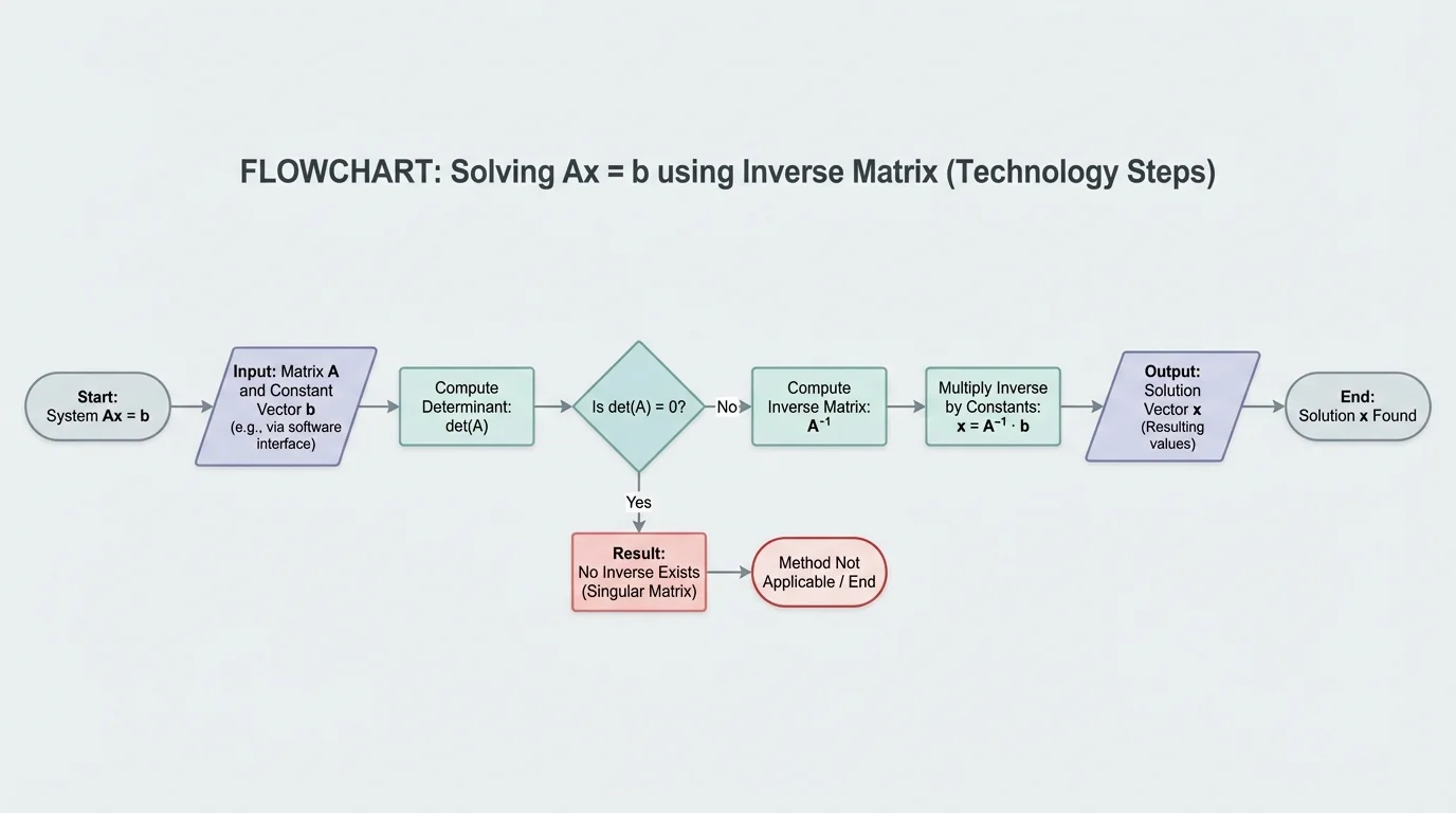
For a \(3 \times 3\) matrix or larger, finding the inverse by hand can become long and error-prone. Technology makes the process practical, and the workflow follows a clear sequence, as shown in [Figure 3].
Most graphing calculators, spreadsheets, and computer algebra systems can compute determinants, inverses, and matrix products. The general steps are:
Step 1: Enter the coefficient matrix \(A\).
Step 2: Compute \(\det(A)\) to check whether the inverse exists.
Step 3: If \(\det(A) \ne 0\), find \(A^{-1}\).
Step 4: Multiply \(A^{-1}\) by the constant vector \(\mathbf{b}\).
Step 5: Interpret the result as the solution vector.
Even when using technology, you still need the mathematics. A calculator can produce numbers, but you must know what they mean. For example, a matrix inverse that contains decimals may represent exact fractions that the device approximates.
As we saw earlier in [Figure 1], the matrix form keeps the roles of coefficients, variables, and constants separate. That structure becomes even more valuable as systems grow larger.
Consider the system
\[\begin{aligned}x + y + z &= 6 \\ 2x - y + 3z &= 14 \\ -x + 4y + z &= 7\end{aligned}\]
Write it as \(A\mathbf{x} = \mathbf{b}\), where
\[A = \begin{bmatrix}1 & 1 & 1 \\ 2 & -1 & 3 \\ -1 & 4 & 1\end{bmatrix}, \qquad \mathbf{b} = \begin{bmatrix}6 \\ 14 \\ 7\end{bmatrix}\]
Solved example 3
Use technology to solve the system by the inverse method.
Step 1: Check whether \(A\) is invertible.
Using technology, \(\det(A) = -21\).
Since \(-21 \ne 0\), the inverse exists.
Step 2: Find \(A^{-1}\) with technology.
A calculator or software gives
\[A^{-1} = \begin{bmatrix}\frac{13}{21} & \frac{1}{7} & -\frac{4}{21} \\ \frac{5}{21} & -\frac{2}{21} & \frac{1}{21} \\ -\frac{1}{3} & \frac{5}{21} & \frac{1}{7}\end{bmatrix}\]
Step 3: Multiply \(A^{-1}\mathbf{b}\).
\[\mathbf{x} = A^{-1}\mathbf{b} = \begin{bmatrix}1 \\ 1 \\ 4\end{bmatrix}\]
Step 4: Interpret the solution.
\[x = 1, \qquad y = 1, \qquad z = 4\]
The system has the unique solution \((1,1,4)\).
A quick substitution check confirms the result: \(1 + 1 + 4 = 6\), \(2(1) - 1 + 3(4) = 14\), and \(-1 + 4(1) + 4 = 7\).
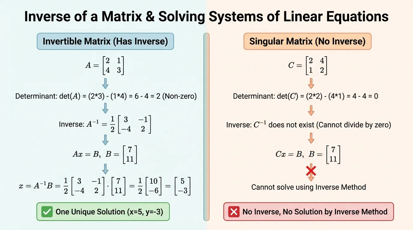
The determinant reveals whether inverse methods can work, as [Figure 4] compares. If \(A\) is invertible, then \(A\mathbf{x} = \mathbf{b}\) has exactly one solution. That is because multiplying by \(A^{-1}\) isolates one and only one vector \(\mathbf{x}\).
If \(A\) is singular, then the inverse does not exist. In that case, the system may have no solution or infinitely many solutions. The inverse method cannot be used because there is no matrix to "undo" the action of \(A\).
This connects matrix algebra to the familiar geometry of lines and planes. In two variables, two lines may intersect once, never intersect, or overlap. In three variables, three planes can also produce one solution, none, or infinitely many. The matrix tells you whether the system is structurally capable of having a unique solution.
Solved example 4
Determine whether the matrix \(B = \begin{bmatrix}2 & 4 \\ 1 & 2\end{bmatrix}\) has an inverse.
Step 1: Compute the determinant.
\(\det(B) = 2 \cdot 2 - 4 \cdot 1 = 4 - 4 = 0\).
Step 2: Interpret the result.
Since \(\det(B) = 0\), the matrix is singular.
Step 3: State the conclusion.
\(B^{-1}\) does not exist.
Any system with coefficient matrix \(B\) cannot be solved by multiplying by an inverse.
This is also why checking the determinant before trying to compute an inverse is a smart habit. It saves time and prevents meaningless work.
One common mistake is multiplying in the wrong order. If \(A\mathbf{x} = \mathbf{b}\), then the correct step is \(A^{-1}A\mathbf{x} = A^{-1}\mathbf{b}\). You multiply on the left, not the right.
Another frequent error is confusing the determinant with the inverse formula. For a \(2 \times 2\) matrix, students often swap entries correctly but forget to divide by \(ad-bc\). That missing factor completely changes the answer.
Technology introduces its own risks. Decimal approximations can hide exact values, and entering one coefficient incorrectly changes the entire solution. As in [Figure 3], the process should always begin with correct matrix entry and a determinant check.
| Issue | What goes wrong | Better habit |
|---|---|---|
| Wrong order | Using \(AA^{-1}\mathbf{b}\) or \(\mathbf{b}A^{-1}\) | Use \(\mathbf{x} = A^{-1}\mathbf{b}\) |
| Skipping determinant | Trying to invert a singular matrix | Check whether \(\det(A) \ne 0\) first |
| Sign error | Incorrect off-diagonal signs in \(2 \times 2\) inverse | Swap diagonal entries and negate off-diagonal entries carefully |
| Technology input error | One wrong entry changes everything | Re-read the matrix before computing |
Table 1. Common mistakes when using inverse matrices and the habits that prevent them.
Inverse matrices are not just an algebra exercise. They are used wherever several unknown quantities must be determined from several relationships.
In economics, a company may produce several products using shared resources such as labor, materials, and machine time. If the total resource use is known, a matrix system can help determine production levels. In network analysis, currents or flows in connected systems can be found by solving simultaneous equations. In chemistry and engineering, mixture problems often lead to linear systems with several variables.
Why technology matters for real systems
Real-world systems are often too large for hand methods. A transportation model, power grid calculation, or data-fitting problem may involve many variables. Matrix methods allow these systems to be organized and solved systematically, while technology handles the heavy computation.
Suppose three ingredients contribute to the amounts of three nutrients in a food blend. If each ingredient contributes known amounts per serving, and the target nutrient totals are known, then the unknown servings can be found from a \(3 \times 3\) system. That is exactly the same structure as \(A\mathbf{x} = \mathbf{b}\).
The big mathematical idea is powerful: when a coefficient matrix has an inverse, the system can be solved cleanly and uniquely. That is why invertibility is one of the most important ideas in linear algebra.