A cup of coffee does not cool in a straight line, and that fact turns out to be mathematically powerful. At first it cools quickly, then more and more slowly, approaching room temperature without ever suddenly flattening out. One familiar function is not always enough to capture that behavior. In many real situations, the best model comes from combining simpler functions into a new one.
When you build a function from other functions, you are doing more than algebraic manipulation. You are deciding what pieces of a situation matter and how they interact. A base amount might stay fixed, while another part changes over time. A cost might include a constant fee plus a variable charge. A medicine level in the body might decay exponentially while another quantity is added at a steady rate. These are all examples of function building.
A single function type often captures only one pattern. A linear function shows a constant rate of change. An exponential function shows repeated percent growth or decay. A constant function stays the same. But many real-world relationships contain more than one pattern at once. A model becomes more realistic when we combine those patterns.
For example, suppose a streaming service charges a fixed monthly fee plus an extra amount per movie rented. The total cost is not just constant and not just linear. It is a constant function added to a linear function. In the same way, the temperature of a cooling object is not just exponential decay. It decays toward a nonzero value, so a constant function must be added to the exponential part.
A function assigns exactly one output to each allowed input. If two functions use the same input variable, such as time, then you can combine their outputs to build a new function.
This idea is one of the main themes in building functions: start with known function types and combine them to describe a relationship between quantities.
Several standard function types appear often in modeling. A constant function has the form \(f(x) = c\). Its output is always the same. A linear function has the form \(f(x) = mx + b\), with a constant rate of change. A quadratic function has the form \(f(x) = ax^2 + bx + c\), which is useful for curved motion and area relationships.
An exponential function has the form \(f(x) = ab^x\), where the input appears in the exponent. If \(0 < b < 1\), the function shows decay. If \(b > 1\), it shows growth. Exponential functions are especially useful when a quantity changes by a constant percentage or when the rate depends on how much remains.
Sometimes a decaying exponential appears in a model together with a constant or linear term. That combination can capture situations that level off, rise from a baseline, or approach a limiting value.
Combined function is a function created by performing arithmetic operations on two or more functions.
Model is a mathematical representation of a relationship between quantities in a real-world situation.
Ambient temperature is the temperature of the surrounding environment, such as the air in a room.
Each function type contributes its own pattern. When you combine them, the new function reflects all those patterns at once.
If \(f(x)\) and \(g(x)\) are functions, then their sum is \((f+g)(x) = f(x) + g(x)\), their difference is \((f-g)(x) = f(x) - g(x)\), their product is \((fg)(x) = f(x)g(x)\), and their quotient is \((f/g)(x) = \dfrac{f(x)}{g(x)}\), as long as \(g(x) \neq 0\).
[Figure 1] Addition combines outputs. If one function represents a base amount and another represents a changing amount, then adding them gives a total. Subtraction can represent a loss, a difference from a baseline, or a net amount. Multiplication can represent scaling or interaction between factors. Division can represent a rate or efficiency.
Domain still matters. If both functions are defined for all real numbers, then their sum, difference, and product are usually also defined for all real numbers. But for a quotient, any input that makes the denominator \(0\) must be excluded.
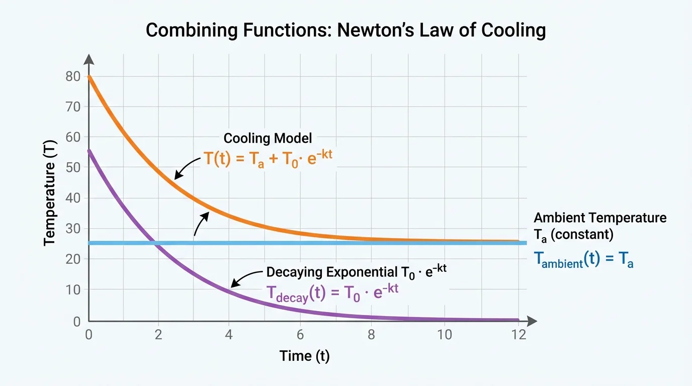
Notice what addition does in the cooling example. If the exponential part approaches \(0\) as time increases, then adding a constant shifts the graph upward so it approaches that constant instead. That is exactly what happens when an object cools toward room temperature rather than toward \(0^\circ\).
Writing a function is only part of the work. You must also explain what each term means. Suppose \(T(t) = 22 + 58(0.8)^t\). The constant \(22\) can represent room temperature in degrees Celsius. The term \(58(0.8)^t\) represents the amount by which the object is still above room temperature after \(t\) hours. At \(t = 0\), the extra temperature is \(58\), and each hour only \(80\%\) of that difference remains.
That interpretation is powerful because it connects algebra to reality. Instead of seeing the function as just symbols, you can identify a baseline, a changing part, an initial amount, and a long-term behavior.
Why the cooling model works
When an object is hotter than its surroundings, the temperature difference between the object and the environment tends to shrink over time. The difference often follows exponential decay, while the surrounding temperature stays constant. So the object's temperature is modeled as constant surrounding temperature + remaining temperature difference.
This pattern appears in many other settings too. A population might approach a carrying level. A bank account might have a fixed monthly deposit plus interest that grows the balance exponentially. A machine might lose value over time but still keep a scrap value that acts like a lower limit.
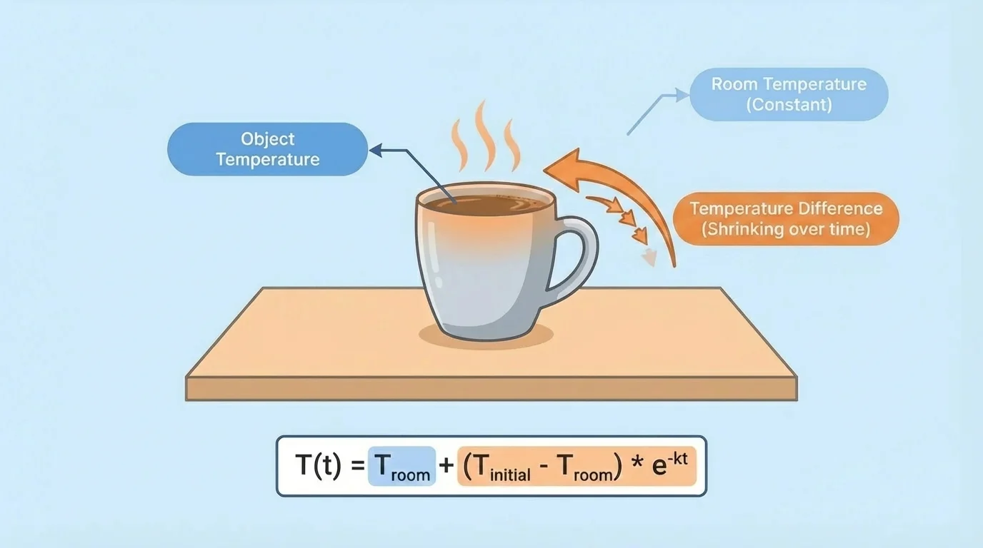
[Figure 2] helps connect the formula to the physical situation of a hot object in a cooler room. A common model for the temperature of a cooling object is \[T(t) = T_a + (T_0 - T_a)b^t\] where \(T_a\) is the ambient temperature, \(T_0\) is the initial temperature of the object, and \(0 < b < 1\).
Here, \(T_a\) is a constant function. The expression \((T_0 - T_a)b^t\) is a decaying exponential function. At \(t = 0\), we get \(T(0) = T_a + (T_0 - T_a) = T_0\), so the model starts at the correct initial temperature. As \(t\) grows, \(b^t\) gets closer to \(0\), so \(T(t)\) gets closer to \(T_a\).
This shows why the model makes sense: the object does not cool forever past room temperature. Instead, the changing part becomes smaller and smaller while the constant ambient temperature remains.
If the room temperature were \(20^\circ\textrm{C}\) and the object started at \(90^\circ\textrm{C}\), then the initial difference would be \(70^\circ\textrm{C}\). If \(b = 0.75\), then every unit of time the difference is multiplied by \(0.75\). The object cools rapidly at first because the difference is large, and more slowly later because the difference has become small.
The best way to learn function building is to connect each algebraic step to a quantity in the situation.
Worked example 1: Writing a cooling model
A metal rod is removed from a furnace at \(180^\circ\textrm{C}\) and placed in a room at \(25^\circ\textrm{C}\). Each minute, the temperature difference between the rod and the room is multiplied by \(0.85\). Write a function for the rod's temperature after \(t\) minutes.
Step 1: Identify the constant part.
The ambient temperature is \(25^\circ\textrm{C}\), so the constant function is \(25\).
Step 2: Find the initial temperature difference.
\(180 - 25 = 155\), so the rod starts \(155^\circ\textrm{C}\) above room temperature.
Step 3: Write the decaying exponential part.
Because \(85\%\) of the difference remains each minute, the difference after \(t\) minutes is \(155(0.85)^t\).
Step 4: Add the constant and changing parts.
\[T(t) = 25 + 155(0.85)^t\]
This function models the rod's temperature over time.
Notice how the model is built from two simpler functions: a constant baseline and a shrinking difference.
Worked example 2: Evaluating a combined function
Use the model \(T(t) = 25 + 155(0.85)^t\) to estimate the rod's temperature after \(4\) minutes.
Step 1: Substitute \(t = 4\).
\(T(4) = 25 + 155(0.85)^4\)
Step 2: Compute the power.
\(0.85^4 = 0.52200625\)
Step 3: Multiply.
\[155(0.52200625) \approx 80.91\]
Step 4: Add the ambient temperature.
\[T(4) \approx 25 + 80.91 = 105.91\]
After \(4\) minutes, the rod's temperature is about \(105.9^\circ\textrm{C}\).
That answer also fits the context: the rod is still hotter than the room, but it has cooled substantially from \(180^\circ\textrm{C}\).
Worked example 3: Building a cost function from two standard types
A delivery company charges a flat service fee of $12 plus $1.80 per mile. Let \(m\) be the number of miles. Write the total cost function and find the cost for \(15\) miles.
Step 1: Write the constant part.
The flat fee is \(12\), so one function is \(f(m) = 12\).
Step 2: Write the linear part.
The mileage charge is \(1.80m\), so another function is \(g(m) = 1.80m\).
Step 3: Add the functions.
\[C(m) = 12 + 1.80m\]
Step 4: Evaluate at \(m = 15\).
\[C(15) = 12 + 1.80(15) = 12 + 27 = 39\]
The delivery cost is $39 for \(15\) miles.
Although this example is linear rather than exponential, the same idea applies: combine simple functions to match the structure of the situation.
Worked example 4: Subtracting functions to model net amount
A theater's ticket revenue is \(R(n) = 14n\), where \(n\) is the number of tickets sold, and operating cost is \(K(n) = 500 + 2n\). Write a function for profit.
Step 1: Recall the relationship.
Profit equals revenue minus cost, so \(P(n) = R(n) - K(n)\).
Step 2: Substitute the functions.
\(P(n) = 14n - (500 + 2n)\)
Step 3: Simplify.
\[P(n) = 12n - 500\]
Subtraction builds a new function that describes net gain instead of total income or total cost alone.
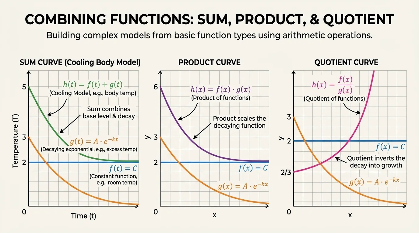
Different arithmetic operations produce different kinds of models. Adding functions often shifts or combines trends, while multiplying and dividing can create much more dramatic changes in shape.
[Figure 3] If \(f(x) = 3\) and \(g(x) = 2^x\), then \((f+g)(x) = 3 + 2^x\) shifts the exponential graph upward by \(3\). But \((fg)(x) = 3 \cdot 2^x\) stretches the exponential vertically. And \((f/g)(x) = \dfrac{3}{2^x}\) creates exponential decay. The operation changes both the graph and the meaning.
In the cooling model, addition is the correct operation because one part represents the fixed surrounding temperature and the other part represents the changing temperature difference. If you multiplied instead, the physical meaning would no longer match the situation.
This is an important modeling principle: do not choose operations just because they are algebraically possible. Choose them because they represent how quantities are related.
Combined functions appear in many fields. In medicine, the concentration of a drug may decay over time while repeated doses add new amounts. In economics, total cost may equal fixed cost plus variable cost. In environmental science, a pollutant level might decline naturally but remain above a background level. In engineering, the temperature of a machine part may cool toward the surrounding air temperature exactly like the model in [Figure 2].
Even personal finance uses the same thinking. A savings balance can be modeled with a constant initial deposit plus growth, or with regular withdrawals subtracted from an increasing amount. Sports analytics, population studies, and physics all rely on combining familiar functions to match real patterns.
Newton's law of cooling helps explain why a hot drink cools quickly at first but much more slowly later. The reason is that the rate of cooling depends on the temperature difference, not just on time itself.
Whenever you read a model, ask two questions: what quantity does each term represent, and why are those terms combined by that specific operation?
One common mistake is confusing the initial value with the long-term value. In \(T(t) = T_a + (T_0 - T_a)b^t\), the initial value is \(T_0\), but the value the function approaches is \(T_a\). Those are not the same unless the object already matches the environment.
Another mistake is choosing the wrong decay factor. If the temperature difference decreases by \(15\%\) each minute, then \(85\%\) remains, so the factor is \(0.85\), not \(0.15\).
Students also sometimes forget to interpret the whole expression. In the model shown earlier in [Figure 1], the exponential part alone does not give the object's actual temperature; it gives the amount above ambient temperature. The full temperature comes only after adding the constant term.
Finally, watch the domain. If time cannot be negative, then the meaningful domain may be \(t \geq 0\), even if the formula itself can accept any real number.
When building a function, start by identifying the quantities and how they behave. Ask whether there is a fixed amount, a constant rate, a repeated percent change, or a curved pattern. Then decide whether the relationship calls for addition, subtraction, multiplication, or division.
A strong model is not just mathematically correct. It also matches the situation, gives sensible values, and allows you to interpret every part of the expression. The cooling model is a great example because every symbol has a clear meaning: environment, starting value, remaining difference, and time.