Companies decide how many products to ship, cities estimate how many buses they need, and streaming services predict how many devices a household may use at once. None of those decisions comes from guessing. They come from data. Probability is not only about coins and dice; it is also about turning real observations into a model that helps us make smart decisions.
In some situations, probabilities are known from symmetry. For a fair die, each outcome has probability \(\dfrac{1}{6}\). But many real-life situations are not symmetric. The number of cars in a family driveway, the number of absences in a week, or the number of TV sets in a household must be estimated from observed data. This is called empirical probability.
Empirical probability is based on what actually happens in collected data. If a survey observes 1,000 households and 260 of them have exactly two TV sets, then the empirical probability of a randomly selected household having two TV sets is \(\dfrac{260}{1000}=0.26\).
These probabilities let us build a mathematical model of a situation. Once the model is built, we can answer useful questions such as: What is the average number of TV sets per household? How many TV sets should we expect among 100 households? What total number is reasonable in the long run?
Sample space is the set of all possible outcomes in a probability situation.
Random variable is a variable whose value depends on the outcome of a chance process.
Probability distribution is a list or table showing each possible value of a random variable and the probability of that value.
When the possible values are countable, such as \(0,1,2,3,4\), we are working with a discrete random variable. In this lesson, the random variables are all discrete because they count things.
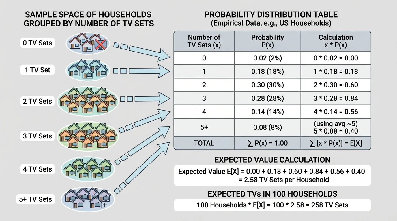
A random variable can take a complicated sample space and turn it into something easier to analyze, as [Figure 1] illustrates. For example, suppose the sample space consists of all households in a survey. Define the random variable \(X\) to be the number of TV sets in a selected household. Then \(X\) might take values such as \(0,1,2,3,4,5\).
A probability distribution for \(X\) tells us the probability attached to each value. For a valid distribution, two rules must hold:
First, every probability must be between \(0\) and \(1\), inclusive.
Second, the probabilities must add up to \(1\):
\[\sum P(x)=1\]
For instance, if \(P(X=0)=0.02\), \(P(X=1)=0.12\), \(P(X=2)=0.27\), \(P(X=3)=0.31\), \(P(X=4)=0.18\), and \(P(X=5)=0.10\), then the distribution is valid because \(0.02+0.12+0.27+0.31+0.18+0.10=1.00\).
This kind of table does not tell us what happens in one specific household. Instead, it describes the pattern across many households. That is why probability distributions are powerful tools for decision-making.
To build a probability distribution from data, we count how often each value occurs, then divide by the total number of observations. This use of relative frequency, as shown in [Figure 2], is the key step in assigning empirical probabilities.
If a data set has \(n\) observations, and the value \(x\) occurs \(f\) times, then
\[P(X=x)=\frac{f}{n}\]
This formula turns raw data into a probability model. The larger the data set, the more reliable the empirical probabilities usually become, because they are based on more evidence.
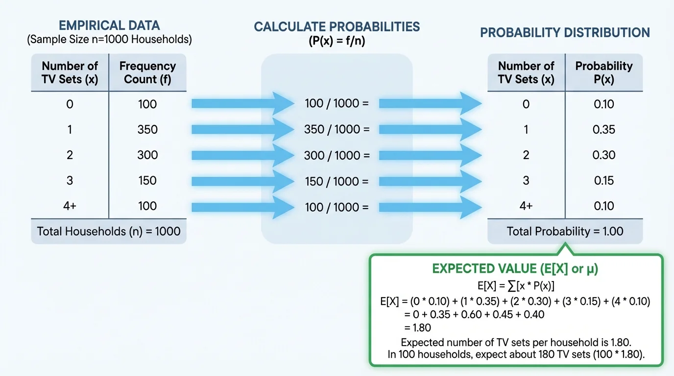
Suppose a survey of \(50\) students records the number of siblings each student has. If \(15\) students have \(2\) siblings, then \(P(X=2)=\dfrac{15}{50}=0.30\). Repeating that for all values gives the full distribution.
Expected value as a weighted average
The expected value is not found by adding all possible values and dividing by how many there are unless each value is equally likely. In a probability distribution, some values occur more often than others, so each value must be weighted by its probability. That is why expected value is a weighted average.
The expected value of a discrete random variable \(X\) is
\[E(X)=\sum xP(x)\]
This formula multiplies each possible value by its probability and then adds the products. If a value is very likely, it contributes more to the expected value. If a value is rare, it contributes less.
Expected value describes the long-run average result over many selections or repetitions. It does not have to be one of the actual values in the distribution. For example, the expected number of TV sets per household might be \(2.67\), even though no single household has exactly \(2.67\) TV sets.
Before looking at the household TV example, let us build and analyze a smaller empirical distribution from scratch.
Example 1: Number of school club memberships
A survey of \(40\) students records the number of clubs each student belongs to. The results are as follows: \(0\) clubs for \(6\) students, \(1\) club for \(14\) students, \(2\) clubs for \(12\) students, \(3\) clubs for \(6\) students, and \(4\) clubs for \(2\) students. Find the probability distribution and the expected number of club memberships.
Step 1: Convert frequencies to probabilities.
Total students: \(40\).
\(P(X=0)=\dfrac{6}{40}=0.15\)
\(P(X=1)=\dfrac{14}{40}=0.35\)
\(P(X=2)=\dfrac{12}{40}=0.30\)
\(P(X=3)=\dfrac{6}{40}=0.15\)
\(P(X=4)=\dfrac{2}{40}=0.05\)
Step 2: Check that the probabilities add to \(1\).
\(0.15+0.35+0.30+0.15+0.05=1.00\)
Step 3: Compute the expected value.
\(E(X)=0(0.15)+1(0.35)+2(0.30)+3(0.15)+4(0.05)\)
\(E(X)=0+0.35+0.60+0.45+0.20=1.60\)
The expected number of club memberships is \(1.6\). Over many students, the average is about \(1.6\) clubs per student.
Notice that \(1.6\) is not the most common value; the most common value is \(1\). Expected value and most likely value are different ideas. The expected value represents the average balance point of the whole distribution.
Now consider a realistic empirical distribution for the number of TV sets in a household. The exact percentages can vary by source and year, but survey data often show that households with \(2\) or \(3\) TV sets are common, while households with \(0\) TV sets are uncommon. The distribution in [Figure 3] gives one representative model suitable for calculation.
| Number of TV sets, \(x\) | Probability, \(P(X=x)\) |
|---|---|
| \(0\) | \(0.02\) |
| \(1\) | \(0.11\) |
| \(2\) | \(0.25\) |
| \(3\) | \(0.30\) |
| \(4\) | \(0.20\) |
| \(5\) | \(0.12\) |
Table 1. An empirical probability distribution for the number of TV sets per household.
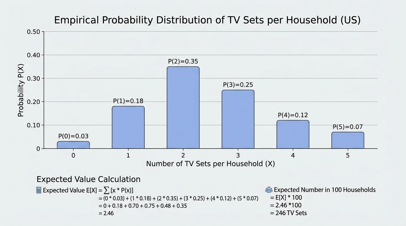
This distribution is valid because the probabilities sum to \(1\): \(0.02+0.11+0.25+0.30+0.20+0.12=1.00\).
Example 2: Expected number of TV sets per household
Use the distribution in Table 1 to find the expected number of TV sets in a randomly selected household.
Step 1: Write the expected value formula.
\(E(X)=\sum xP(x)\)
Step 2: Multiply each value by its probability.
\(0(0.02)=0\)
\(1(0.11)=0.11\)
\(2(0.25)=0.50\)
\(3(0.30)=0.90\)
\(4(0.20)=0.80\)
\(5(0.12)=0.60\)
Step 3: Add the products.
\(E(X)=0+0.11+0.50+0.90+0.80+0.60=2.91\)
The expected number of TV sets per household is \(2.91\).
This means that if we selected many households and averaged their numbers of TV sets, the mean would be about \(2.91\). The distribution is centered near \(3\), so an expected value slightly below \(3\) makes sense.
Expected value becomes especially useful when we scale up from one selection to many. If the expected number of TV sets in one household is \(2.91\), then in \(100\) randomly selected households, the expected total number of TV sets is
\[100(2.91)=291\]
So we would expect to find about \(291\) TV sets in \(100\) randomly selected households.
This works because averages scale linearly. If the average per household is \(2.91\), then multiplying by the number of households gives the expected total. This does not mean every group of \(100\) households will have exactly \(291\) TV sets, but it is the long-run average you would predict.
When you multiply an average per item by the number of items, you get an expected total. This idea is the same one used when estimating total cost from average cost, or total distance from average distance per trip.
If you sampled another set of \(100\) households, the total might be \(286\), \(294\), or \(300\). Random variation causes totals to change from sample to sample. Expected value tells you the center of those possible totals, not the exact total every time.
Students often think expected value means "the answer most likely to happen." That is not always true. In the TV-set distribution, the most likely value is \(3\), because \(P(X=3)=0.30\) is the largest probability. But the expected value is \(2.91\), which is not exactly the same.
The expected value also might not be a possible outcome at all. A family cannot own \(2.91\) TV sets. But a distribution can still have an expected value of \(2.91\) because expected value is an average over many households.
Another useful idea is that expected value is sensitive to larger values. Even if only a smaller percentage of households have \(5\) TV sets, that category still pulls the average upward because \(5\) is a large contribution in the product \(xP(x)\).
Different situations follow the same structure: define the random variable, assign empirical probabilities from data, and compute \(E(X)\).
Example 3: Number of books checked out
At a school library, data from \(80\) students show the following numbers of books checked out in a week: \(0\) books for \(20\) students, \(1\) book for \(28\) students, \(2\) books for \(18\) students, \(3\) books for \(10\) students, and \(4\) books for \(4\) students. Find the expected number of books checked out per student.
Step 1: Write probabilities from the frequencies.
\(P(0)=\dfrac{20}{80}=0.25\), \(P(1)=\dfrac{28}{80}=0.35\), \(P(2)=\dfrac{18}{80}=0.225\), \(P(3)=\dfrac{10}{80}=0.125\), \(P(4)=\dfrac{4}{80}=0.05\)
Step 2: Calculate the expected value.
\(E(X)=0(0.25)+1(0.35)+2(0.225)+3(0.125)+4(0.05)\)
\(E(X)=0+0.35+0.45+0.375+0.20=1.375\)
The expected number of books checked out is \(1.375\), or about \(1.38\) books per student.
Because expected value gives a long-run average, the library can use this result to estimate total circulation. For \(500\) students, the expected total number of books checked out is about \(500(1.375)=687.5\), so around \(688\) books would be a reasonable estimate.
Example 4: Number of late arrivals per day
A school office tracks late arrivals over \(50\) days. The counts are: \(0\) late arrivals on \(8\) days, \(1\) on \(17\) days, \(2\) on \(13\) days, \(3\) on \(9\) days, and \(4\) on \(3\) days. Find the expected number of late arrivals per day.
Step 1: Convert to probabilities.
\(P(0)=\dfrac{8}{50}=0.16\)
\(P(1)=\dfrac{17}{50}=0.34\)
\(P(2)=\dfrac{13}{50}=0.26\)
\(P(3)=\dfrac{9}{50}=0.18\)
\(P(4)=\dfrac{3}{50}=0.06\)
Step 2: Compute the expected value.
\(E(X)=0(0.16)+1(0.34)+2(0.26)+3(0.18)+4(0.06)\)
\(E(X)=0+0.34+0.52+0.54+0.24=1.64\)
The expected number of late arrivals is \(1.64\) per day.
If administrators want to estimate the total number of late arrivals over a \(180\)-day school year, they can use \(180(1.64)=295.2\), so about \(295\) late arrivals would be expected.
Expected values are used in fields as different as sports strategy, insurance pricing, public health planning, and online recommendation systems. Whenever experts balance likely outcomes with their probabilities, they are using this same idea.
Insurance companies use empirical distributions to estimate how much they will need to pay in claims. Manufacturers use them to estimate how many defective items might appear in a production run. Hospitals may estimate the expected number of patients arriving in a certain time period. In each case, one observed value is not enough. The power comes from the distribution of many outcomes.
Expected value also supports decision-making. Suppose a city wants to estimate how many parking spaces are needed in a neighborhood. If survey data show an expected value of \(1.8\) cars per household and there are \(2{,}000\) households, then the expected total is \(2{,}000(1.8)=3{,}600\) cars. That estimate helps planners make practical choices.
The same logic that helped us predict around \(291\) TV sets in \(100\) households applies in all these cases. A carefully built empirical probability distribution turns real data into a model for informed decisions.
One common mistake is forgetting to divide by the total number of observations when turning frequencies into probabilities. Frequencies are counts; probabilities are proportions.
Another mistake is forgetting to check that probabilities add to \(1\). If they do not, the distribution is not valid and the expected value calculation will be wrong.
A third mistake is calculating the ordinary mean of the possible values without using probabilities. For example, averaging \(0,1,2,3,4,5\) gives \(\dfrac{0+1+2+3+4+5}{6}=2.5\), but that only works if all six values are equally likely. In empirical distributions, they usually are not.
Finally, do not confuse the expected value with the most likely value. The expected value is a weighted average, while the most likely value is the one with the greatest probability.