One of the most powerful ideas in algebra is that you can change the appearance of a problem without changing its answer. That is exactly what happens in elimination: an equation may look different after you add a multiple of another equation to it, but the system can still describe the very same solution. This is not just a convenient trick. It is a fact that can be proved carefully, and that proof explains why elimination is a valid method rather than a lucky shortcut.
When you solve a system of two equations in two variables, you are looking for all ordered pairs \( (x,y) \) that make both equations true at the same time. A system may have one solution, no solution, or infinitely many solutions. In every case, the methods you use must preserve the set of solutions.
If you start with one system and transform it into another system, the new system is called an equivalent system if both systems have exactly the same solutions. The elimination method works because certain operations create equivalent systems. The most important of these is replacing one equation by the sum of that equation and a multiple of the other.
To solve a system means to find every ordered pair \( (x,y) \) that satisfies each equation in the system. If an ordered pair makes one equation true but not the other, it is not a solution to the system.
Before proving the rule, it helps to name the main ideas clearly. The proof itself is short, but the meaning behind it is deep: algebra lets you rewrite information in a form that is easier to use while keeping the same mathematical truth.
System of equations: a collection of equations considered together, such as \(a_1x+b_1y=c_1\) and \(a_2x+b_2y=c_2\).
Solution: an ordered pair \( (x,y) \) that makes every equation in the system true.
Equivalent systems: two systems that have exactly the same solution set.
Suppose a system is
\[\begin{cases} E_1 \\ E_2 \end{cases}\]
where \(E_1\) and \(E_2\) are equations in \(x\) and \(y\). Choose any real number \(k\). The rule says that if you replace \(E_1\) by \(E_1+kE_2\), then the new system
\[\begin{cases} E_1+kE_2 \\ E_2 \end{cases}\]
has the same solutions as the original system. The same idea works if you replace \(E_2\) by \(E_2+kE_1\).
This is the algebraic foundation of elimination. When students multiply one equation and add it to the other, they are using this exact principle.
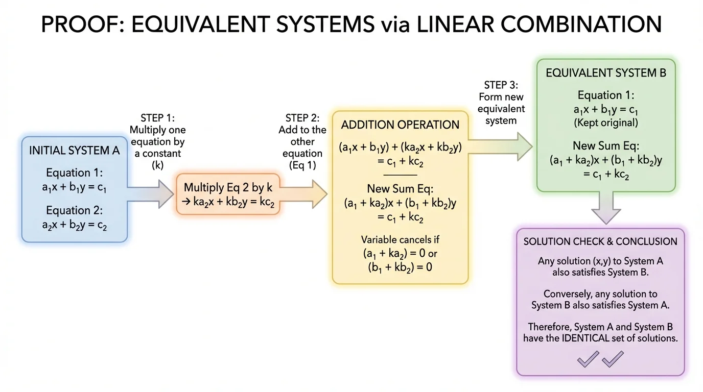
Now we prove the statement in general form. Let the original system be
\[\begin{cases} a_1x+b_1y=c_1 \\ a_2x+b_2y=c_2 \end{cases}\]
and let \(k\) be any real number. Replace the first equation with the sum of the first equation and \(k\) times the second equation. The new system is
\[\begin{cases} (a_1+ka_2)x+(b_1+kb_2)y=c_1+kc_2 \\ a_2x+b_2y=c_2 \end{cases}\]
To prove the two systems are equivalent, we must show two things: every solution of the original system is a solution of the new system, and every solution of the new system is a solution of the original system.
The two-way proof idea
When proving two systems have the same solutions, one direction is not enough. You must show that solutions can move from the original system to the new one, and also back from the new system to the original one. That is what guarantees the solution sets are identical.
First direction: assume \( (x,y) \) is a solution of the original system. Then
\[a_1x+b_1y=c_1 \quad \textrm{and} \quad a_2x+b_2y=c_2\]
Since the second equation is true, multiplying it by \(k\) gives
\[ka_2x+kb_2y=kc_2\]
Now add this to the first equation:
\[(a_1x+b_1y)+(ka_2x+kb_2y)=c_1+kc_2\]
which simplifies to
\[(a_1+ka_2)x+(b_1+kb_2)y=c_1+kc_2\]
This is exactly the new first equation, and the second equation is still \(a_2x+b_2y=c_2\), which was already true. So \( (x,y) \) solves the new system.
Second direction: assume \( (x,y) \) is a solution of the new system. Then
\[(a_1+ka_2)x+(b_1+kb_2)y=c_1+kc_2\]
and
\[a_2x+b_2y=c_2\]
Multiply the second equation by \(-k\):
\[-ka_2x-kb_2y=-kc_2\]
Add this to the new first equation:
\[((a_1+ka_2)x+(b_1+kb_2)y)+(-ka_2x-kb_2y)=(c_1+kc_2)+(-kc_2)\]
After simplifying, you get
\[a_1x+b_1y=c_1\]
That is the original first equation. The second equation remains \(a_2x+b_2y=c_2\), so \( (x,y) \) solves the original system as well.
Since each solution of one system is also a solution of the other, the two systems have the same solution set. Therefore, replacing one equation by the sum of that equation and a multiple of the other produces an equivalent system.
Adding a multiple of one equation to another changes the form of a system, not its solution set.
[Figure 1] This proof is simple but important. It tells you that elimination is not based on guesswork. It is based on preserving logical equivalence.
The elimination method uses the proven rule strategically: choose a multiple so that when one equation is added to the other, one variable cancels. The sequence of moves is valid because each replacement produces an equivalent system.
For example, if a system contains \(3x+2y=7\) and \(5x-2y=9\), adding the equations gives \(8x=16\), so \(x=2\). The variable \(y\) disappears because \(2y+(-2y)=0\). This cancellation is not magic; it is the deliberate result of replacing one equation by a sum that preserves all solutions.
Once one variable is eliminated, the system becomes much easier to solve. Then you substitute back to find the other variable. Every algebra class uses this process, but the proof above explains why it is trustworthy.
You can also think of elimination as rewriting the same information in a more useful form. Instead of carrying two equations that are hard to solve together, you transform one into an equation that isolates a variable or removes one entirely.
Consider the system
\[\begin{cases} x+y=5 \\ x-y=1 \end{cases}\]
Worked example
Replace the first equation by itself plus the second equation, then compare the solution sets.
Step 1: Form the new first equation.
Add \(x+y=5\) and \(x-y=1\): \(2x=6\).
The new system is
\[\begin{cases} 2x=6 \\ x-y=1 \end{cases}\]
Step 2: Solve the new system.
From \(2x=6\), we get \(x=3\).
Substitute into \(x-y=1\): \(3-y=1\), so \(y=2\).
Step 3: Check in the original system.
In \(x+y=5\), substituting \(x=3\) and \(y=2\) gives \(3+2=5\), true.
In \(x-y=1\), substituting gives \(3-2=1\), also true.
The original and new systems both have the same solution: \( (3,2) \).
This example shows the rule in action with the simplest possible arithmetic. The first equation changed a lot, but the solution did not change at all.
Now consider a system where a multiple is needed before adding:
\[\begin{cases} 2x+3y=13 \\ x-3y=-2 \end{cases}\]
Worked example
Use replacement to eliminate \(y\).
Step 1: Choose the replacement.
The \(y\)-coefficients are \(3\) and \(-3\), so adding the equations will eliminate \(y\). Replace the first equation by the sum of the two equations.
Step 2: Add the equations.
\[(2x+3y)+(x-3y)=13+(-2)\]
This simplifies to \(3x=11\).
The new system is
\[\begin{cases} 3x=11 \\ x-3y=-2 \end{cases}\]
Step 3: Solve for \(x\).
\(x=\dfrac{11}{3}\).
Step 4: Substitute to find \(y\).
Using \(x-3y=-2\):
\[\frac{11}{3}-3y=-2\]
Subtract \(\dfrac{11}{3}\) from both sides:
\[-3y=-2-\frac{11}{3}=-\frac{6}{3}-\frac{11}{3}=-\frac{17}{3}\]
So \(y=\dfrac{17}{9}\).
The solution is \(\left(\dfrac{11}{3},\dfrac{17}{9}\right)\).
The reason this method is valid is exactly the theorem proved earlier. We replaced one equation by the sum of that equation and a multiple of the other, so we never changed the solution set.
The rule also works when a system is inconsistent. Consider
\[\begin{cases} x+y=4 \\ 2x+2y=10 \end{cases}\]
Worked example
Replace the second equation by itself minus \(2\) times the first equation.
Step 1: Compute the replacement.
Start with the second equation, \(2x+2y=10\). Twice the first equation is \(2x+2y=8\).
Then
\[(2x+2y)-(2x+2y)=10-8\]
so \(0=2\).
Step 2: Interpret the result.
The new system is
\[\begin{cases} x+y=4 \\ 0=2 \end{cases}\]
The statement \(0=2\) is false for every value of \(x\) and \(y\).
Therefore the system has no solution.
Notice what happened: the replacement did not accidentally create the contradiction. It revealed a contradiction that was already hidden in the original system. Since equivalent systems have the same solutions, an inconsistent system stays inconsistent after a valid replacement.
A system can fail to have a solution even when both equations look perfectly reasonable by themselves. The problem is not with either equation alone; it is that no single ordered pair satisfies both at once.
This is one reason elimination is so useful. It can expose inconsistency quickly by reducing a system to a statement like \(0=2\).
Now consider a dependent system:
\[\begin{cases} x+2y=6 \\ 2x+4y=12 \end{cases}\]
Worked example
Replace the second equation by itself minus \(2\) times the first equation.
Step 1: Compute the replacement.
Twice the first equation is \(2x+4y=12\). Subtract this from the second equation:
\[(2x+4y)-(2x+4y)=12-12\]
So the new equation is \(0=0\).
Step 2: Interpret the result.
The new system is
\[\begin{cases} x+2y=6 \\ 0=0 \end{cases}\]
The equation \(0=0\) is always true, so the system is really described by just \(x+2y=6\).
Step 3: Describe the solutions.
Let \(y=t\), where \(t\) is any real number. Then \(x=6-2t\).
The system has infinitely many solutions, given by \( (x,y)=(6-2t,t) \) for all real \(t\).
Again, the replacement preserved the solution set. The equation \(0=0\) shows that one equation was a multiple of the other, so both equations represent the same line.
This replacement rule has several useful variations. First, the multiple can be any real number \(k\), including fractions and negative numbers. For example, replacing an equation by itself plus \(\dfrac{1}{2}\) of the other is completely valid.
Second, if \(k=0\), then nothing changes. Replacing an equation by itself plus \(0\) times the other leaves the equation unchanged. This fits the rule perfectly.
Third, you may replace either equation. If the system is
\[\begin{cases} E_1 \\ E_2 \end{cases}\]
then both
\[\begin{cases} E_1+kE_2 \\ E_2 \end{cases}\quad \textrm{and} \quad \begin{cases} E_1 \\ E_2+kE_1 \end{cases}\]
are equivalent to the original system.
A closely related idea appears in row operations for matrices. One legal row operation is replacing one row by itself plus a multiple of another row. The theorem you proved for equations is the same idea in a different language.
There is also an important limit to remember: you must keep one original equation while replacing the other. The theorem is about a specific valid move. If you perform several moves in a row, that is fine, as long as each move is valid and each new system is equivalent to the one before it.
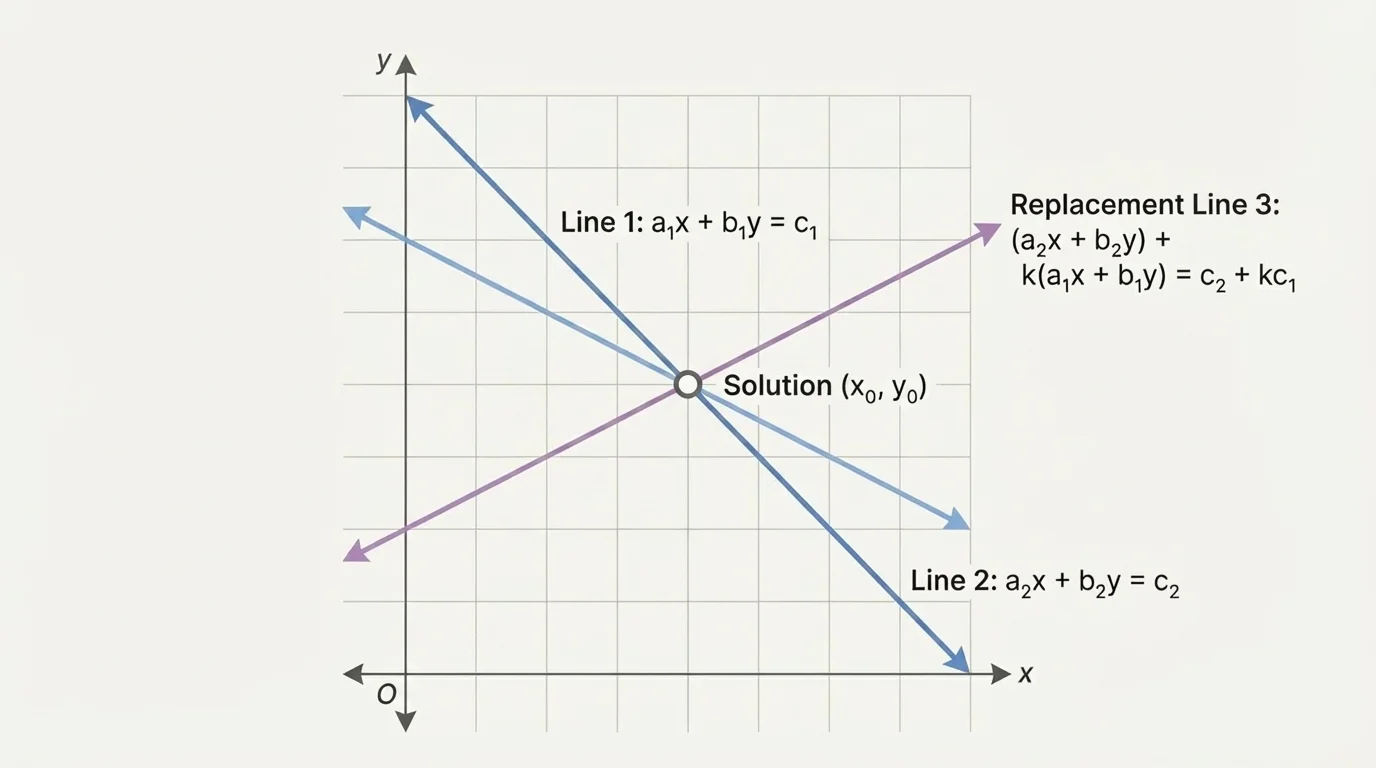
[Figure 2] Systems of two linear equations can be viewed as pairs of lines in the coordinate plane. The solution is the point where the lines intersect, if they intersect at all.
[Figure 2] shows that a replacement equation can look different from the original one while still passing through exactly the same intersection point with the unchanged line.
Suppose a point \( (x,y) \) lies on both original lines. Then it satisfies both equations. Because it satisfies both, it also satisfies any sum of one equation with a multiple of the other. So the intersection point remains on the new line. That is the geometric reason the solution set stays the same.
If the original lines are parallel and never meet, a valid replacement will still produce a system with no common point. If the original equations describe the same line, the replacement will still describe that same entire set of points. So the three possible outcomes—one solution, no solution, or infinitely many solutions—are all preserved.
Later, when you think back to [Figure 2], it helps to remember that equations in an equivalent system do not have to look identical. What matters is whether they describe the same common set of solutions together with the other equation.
In engineering, economics, and science, systems of equations are often rewritten into easier forms before solving. For example, two measured quantities might produce a pair of equations in unknown values such as cost, speed, or concentration. Scientists and engineers routinely combine equations to eliminate a variable and isolate the quantity they want.
Suppose two chemical mixtures have concentrations that lead to a system of linear equations in the amounts of two substances. A technician may multiply one equation and add it to another to remove one variable and solve more efficiently. The validity of that step depends on the same theorem: the transformed system must preserve the original solution set.
Economists do something similar when comparing two linear constraints in a model. The equations may be rewritten to expose a key relationship without changing the actual feasible solution. Algebra is not only about symbols on paper; it is a way of preserving truth while making information more usable.
One common error is adding equations incorrectly, especially with negative signs. For instance, \(-3y+3y=0\), not \(6y\). Since elimination depends on careful cancellation, sign errors can completely change the result.
Another mistake is replacing an equation and then continuing to use the old version of that same equation as if nothing changed. Once you replace an equation, the new system contains the replacement equation and the unchanged other equation.
A third mistake is believing that a contradiction like \(0=5\) means you made an error automatically. Sometimes it does indicate an arithmetic mistake, but sometimes it correctly shows that the system has no solution. Similarly, a result like \(0=0\) may correctly show infinitely many solutions.
Finally, remember that the proof depends on logical equivalence. You are not trying random manipulations; you are using a theorem that guarantees the same solutions are preserved at every valid step.
The key theorem can be stated in one sentence: if you replace one equation in a two-variable system by the sum of that equation and a multiple of the other, the new system is equivalent to the original. The proof works in both directions, and that two-way logic is what makes elimination a rigorous algebraic method.
Whenever you eliminate a variable, you are relying on this fact. It is one of the clearest examples in algebra of how a transformation can change the form of a problem while leaving its meaning exactly the same.