A car slows down at a red light, a phone battery runs a speaker, and a dropped backpack speeds up as it falls. These situations look very different, but they are all governed by the same powerful idea: energy is conserved. What changes is where the energy is stored and how it moves. Once you know the energy change of some parts of a system and any energy entering or leaving, you can calculate the missing change for another part. That is exactly what a computational model does: it turns a physical situation into a clear set of quantities and relationships that can be solved.
In physical science, energy is treated as a quantitative property. That means it can be measured, compared, added, and subtracted. For many grade-level problems, the goal is not to derive advanced formulas but to keep careful track of energy in systems with two or three components. If the accounting is done correctly, the total energy change of the system must match the net energy transferred into or out of the system.
Engineers, scientists, and technicians constantly use energy accounting. A mechanical engineer checks how much kinetic energy a moving machine loses and how much thermal energy the brakes gain. A building designer estimates how energy enters and leaves a room to predict temperature change. A medical device designer tracks electrical energy from a battery and where it ends up in a sensor or heating element. In each case, the central question is the same: if some energy changes are known, what is the unknown change?
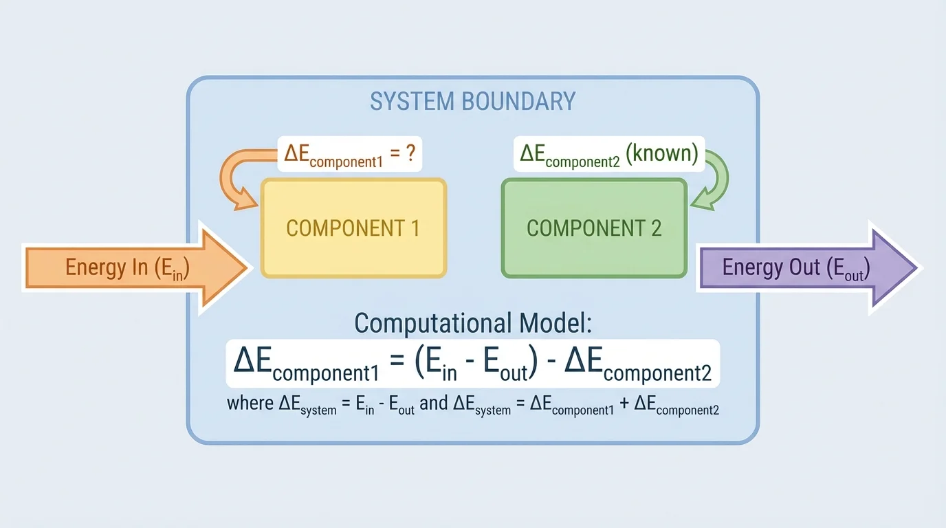
This kind of reasoning works best when we clearly identify the object of study as a system. A system is the part of the world we choose to analyze. Everything outside it is the surroundings. The way we draw the system boundary determines whether an energy change counts as happening inside the system or as energy transferred across the boundary, as [Figure 1] shows in a simple two-component setup. That choice matters because the same physical event can be described in different correct ways depending on what is included in the system.
A system may contain one object or several connected parts. In this lesson, we focus on systems with two or three components, because that is enough to show the logic of conservation without making the calculations too complicated. A component might be a moving cart, the Earth, a brake pad, a battery, or a resistor.
Suppose a ball falls toward Earth. One useful system has two components: the ball and Earth. As the ball falls, the energy stored in the gravitational field changes and the ball's kinetic energy changes. If air resistance is ignored, there may be essentially no energy crossing the system boundary. But if we choose a different system that contains only the ball, then gravity from Earth acts from outside the system, and energy is transferred into the system instead. Both descriptions can work, but the boundary must be chosen carefully and used consistently.
System is the collection of components being analyzed.
Component is one distinct part of the system whose energy can change.
Energy transfer is energy moving into or out of the system across its boundary.
Energy change is the increase or decrease in energy stored by a component or by the system as a whole.
When solving problems, it helps to name each component and assign a variable to each energy change. For a two-component system, you might write the changes as \(\Delta E_1\) for component 1 and \(\Delta E_2\) for component 2. If energy enters the system, call it \(E_{in}\); if energy leaves, call it \(E_{out}\). A computational model is then built from those quantities.
The key principle is conservation of energy, and [Figure 2] illustrates the bookkeeping idea: the total change in energy of the system equals the net energy transferred into the system. For a system with components, that means we add the energy changes of all components and set that sum equal to energy in minus energy out.
The main relationship is
\[\Delta E_{system} = E_{in} - E_{out}\]
and for a system with two components,
\[\Delta E_1 + \Delta E_2 = E_{in} - E_{out}\]
For a system with three components,
\[\Delta E_1 + \Delta E_2 + \Delta E_3 = E_{in} - E_{out}\]
If one component's energy change is unknown, solve for it using basic algebra. For example, in a two-component system,
\[\Delta E_1 = E_{in} - E_{out} - \Delta E_2\]
This equation is the heart of the computational model. It does not matter whether the energy changes involve thermal energy, kinetic energy, or field energy. The structure stays the same. What changes is the physical meaning of each term.
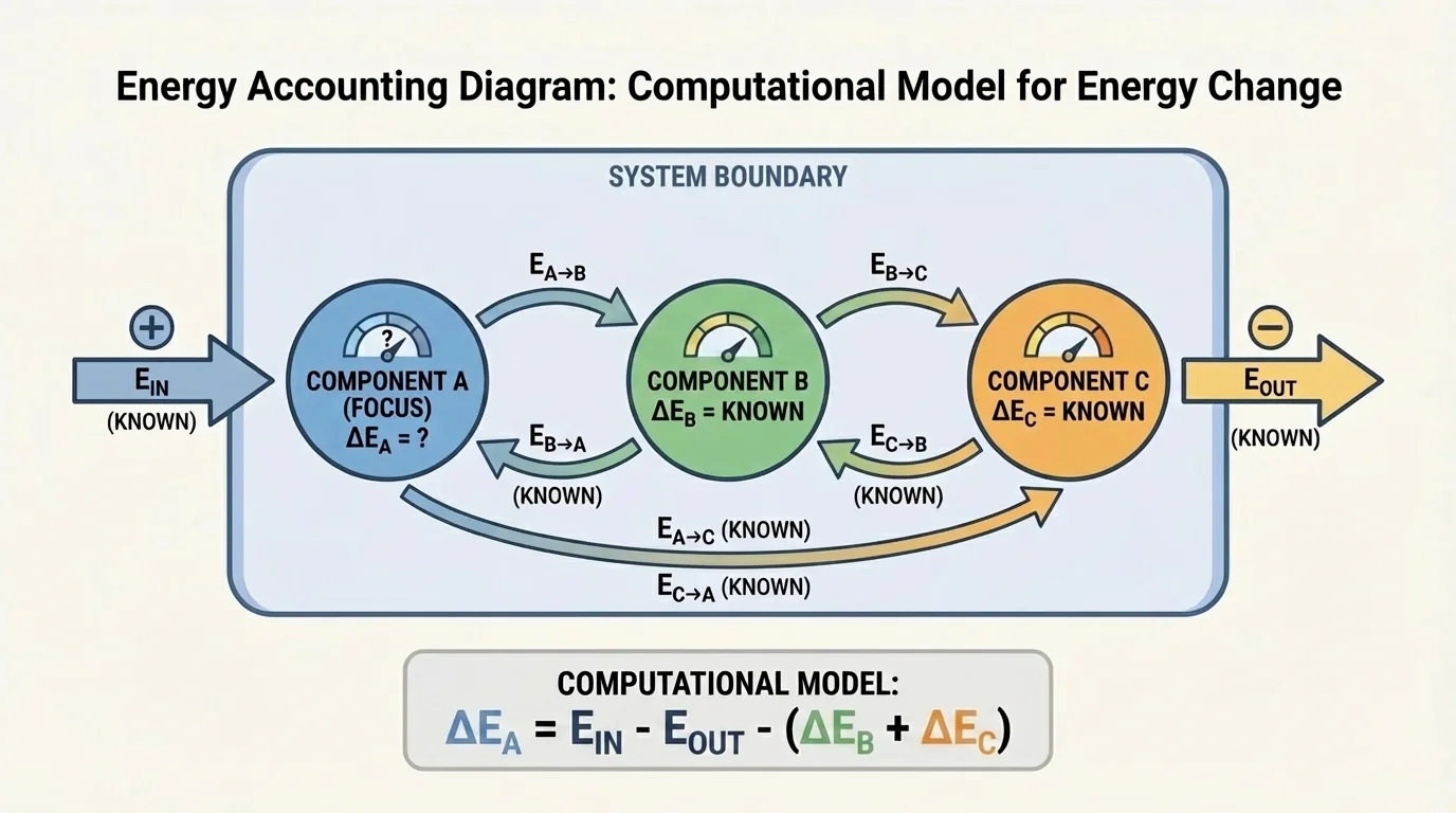
Notice an important idea: energy transfers between components inside the system do not count as energy entering or leaving the system. They may explain why one component gains energy while another loses energy, but they are internal to the system. Only energy crossing the boundary appears as \(E_{in}\) or \(E_{out}\).
The sign convention
A positive energy change means a component gains energy. A negative energy change means a component loses energy. Energy entering the system is treated as positive in the net transfer term, and energy leaving the system is treated as negative through subtraction in the expression \(E_{in} - E_{out}\).
This sign convention is what makes the equations work consistently. If a moving object slows down, its kinetic energy change is negative. If brakes warm up, their thermal energy change is positive. If energy escapes to the surroundings as heat, that amount appears in \(E_{out}\).
A computational model is a simplified mathematical representation of a real situation. In this topic, it can be as simple as a variable equation or a short algorithm. The idea is to organize known values, apply the conservation rule, and compute the unknown quantity.
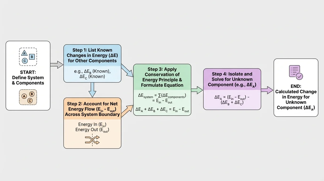
A practical model often follows four steps:
Step 1: Define the system and its components.
Step 2: List each known energy change and each known energy flow into or out of the system.
Step 3: Write the conservation equation.
Step 4: Solve for the unknown and check whether the sign and size make physical sense.
If a battery-powered heater is inside your system and electrical energy enters from outside, you include that as \(E_{in}\). If the system contains the battery itself, then the battery's energy decreases inside the system, and the transfer from the battery to another component is internal. That is why defining the system first is so important.
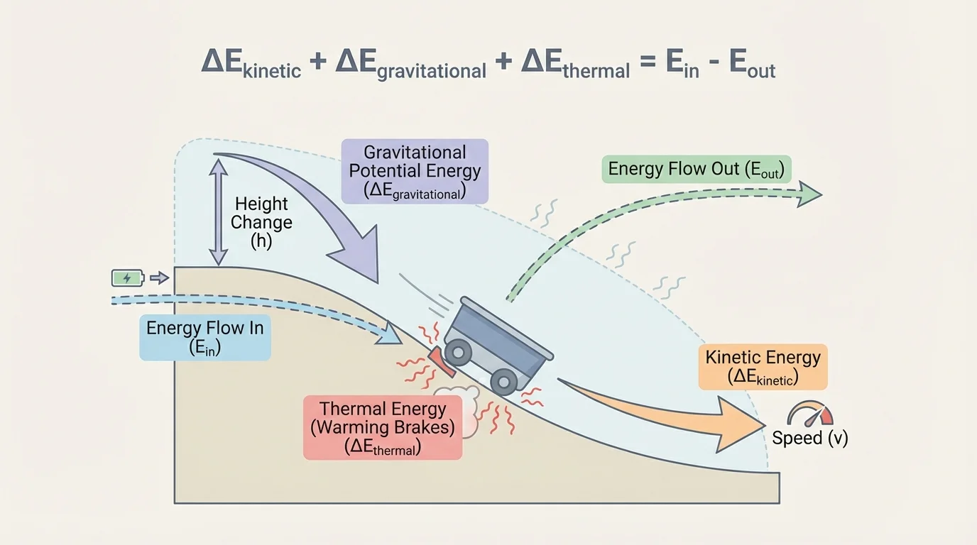
Several energy types are especially useful at this level, and [Figure 3] shows how more than one can change in a single event. You do not need one universal formula for all of them in order to do energy accounting. Often the problem gives the energy changes directly, and you use conservation to find the missing one.
Thermal energy is associated with the random motion and interactions of particles. If an object warms up, its thermal energy increases. If it cools down, its thermal energy decreases.
Kinetic energy is associated with motion. A faster object has more kinetic energy than a slower one. If a cart speeds up, \(\Delta E_k > 0\); if it slows down, \(\Delta E_k < 0\).
Gravitational field energy depends on position in a gravitational field. When an object moves higher above Earth, gravitational field energy increases. When it falls, gravitational field energy decreases.
Electric field energy can change when electric charges move in electric systems, such as batteries and circuits. At this level, you may track the gain or loss of electric energy without using advanced circuit analysis.
Magnetic field energy can change in systems involving magnets or electromagnets. Again, the key idea is not a complicated formula but careful accounting of what energy increases, decreases, enters, or leaves.
Modern hybrid cars rely heavily on energy accounting. During braking, some of the car's kinetic energy is transformed and stored instead of being lost entirely as thermal energy, which improves efficiency.
The same event can involve several forms of energy at once. A bike rolling downhill may lose gravitational field energy, gain kinetic energy, and also increase thermal energy slightly because of friction. A correct model keeps all relevant terms and does not assume that all lost energy from one component goes into just one other place unless the problem states that.
Now we apply the model to specific cases. Each example uses only basic algebra and systems of two or three components.
Example 1: Two-component thermal system
A hot metal block and cooler water are inside an insulated container. The system has two components: the block and the water. The block's energy change is \(-120 \textrm{ J}\), and no energy enters or leaves the system, so \(E_{in} = 0\) and \(E_{out} = 0\). Find the water's energy change.
Step 1: Write the conservation equation for two components.
\(\Delta E_{block} + \Delta E_{water} = E_{in} - E_{out}\)
Step 2: Substitute known values.
\((-120) + \Delta E_{water} = 0 - 0\)
Step 3: Solve.
\(\Delta E_{water} = 120 \textrm{ J}\)
The water gains \(120 \textrm{ J}\) of thermal energy.
This answer makes physical sense: the hot block loses energy, and the water gains the same amount because no energy escapes the insulated system.
Example 2: Falling object with some energy leaving the system
A system contains a falling ball and Earth. During the fall, the gravitational field energy changes by \(-50 \textrm{ J}\). Air resistance causes \(8 \textrm{ J}\) of energy to leave the system as thermal energy to the surroundings. Find the ball's kinetic energy change.
Step 1: Identify components and transfers.
\(\Delta E_g = -50 \textrm{ J}\), \(\Delta E_k = ?\), \(E_{in} = 0\), \(E_{out} = 8 \textrm{ J}\)
Step 2: Write the equation.
\(\Delta E_g + \Delta E_k = E_{in} - E_{out}\)
Step 3: Substitute and solve.
\((-50) + \Delta E_k = 0 - 8\)
\((-50) + \Delta E_k = -8\)
\(\Delta E_k = 42 \textrm{ J}\)
The ball's kinetic energy increases by \(42 \textrm{ J}\).
The result is smaller than \(50 \textrm{ J}\) because some energy leaves the system instead of all of it becoming kinetic energy. This is exactly the kind of detail that a computational model captures well.
Example 3: Three-component braking system
A system contains a moving bicycle wheel, brake pads, and surrounding air near the brakes. The wheel loses \(200 \textrm{ J}\) of kinetic energy. The brake pads gain \(140 \textrm{ J}\) of thermal energy. Find the energy change of the nearby air if no energy enters or leaves the system.
Step 1: Write the three-component equation.
\(\Delta E_{wheel} + \Delta E_{pads} + \Delta E_{air} = E_{in} - E_{out}\)
Step 2: Substitute values.
\((-200) + 140 + \Delta E_{air} = 0\)
Step 3: Solve.
\(-60 + \Delta E_{air} = 0\)
\(\Delta E_{air} = 60 \textrm{ J}\)
The nearby air gains \(60 \textrm{ J}\) of thermal energy.
This example shows why three-component systems are useful. Not all the wheel's lost kinetic energy goes into the brake pads. Some goes into the air as well.
Example 4: Electric energy in a device
A system contains a battery and a small motor. During operation, the battery's energy change is \(-90 \textrm{ J}\), and the motor's kinetic energy increases by \(55 \textrm{ J}\). Find the net energy leaving the system as thermal energy and sound if no energy enters the system.
Step 1: Use the system equation.
\(\Delta E_{battery} + \Delta E_{motor} = E_{in} - E_{out}\)
Step 2: Substitute values.
\((-90) + 55 = 0 - E_{out}\)
Step 3: Solve.
\(-35 = -E_{out}\)
\(E_{out} = 35 \textrm{ J}\)
\(35 \textrm{ J}\) leaves the system.
That lost energy often appears as warming of parts and sound in real devices. As we saw earlier in [Figure 3], one visible motion change can hide several less obvious energy changes happening at the same time.
A very common error is mixing up energy change with energy transfer. If a component inside the system loses energy, that is written as a negative \(\Delta E\) for that component. It does not automatically mean energy left the system. It may simply have moved to another component inside the boundary.
Another common mistake is forgetting that \(E_{out}\) is subtracted in the equation \(E_{in} - E_{out}\). If \(E_{out} = 12 \textrm{ J}\), then the net transfer term is \(0 - 12 = -12 \textrm{ J}\), not \(12 \textrm{ J}\). That negative result means the system as a whole lost energy to the surroundings.
Students also sometimes double count. For example, if a moving object slows down and a brake warms up, do not count the same energy both as a positive change in the brake and as \(E_{out}\) unless some of that energy actually crosses the boundary into the surroundings.
From earlier work with algebra, solving for an unknown means isolating the variable. If \(a + x = b\), then \(x = b - a\). The same algebraic idea is used in all of the energy equations in this topic.
A quick reasonableness check helps. If one component loses energy and there is no energy entering the system, then the other components together should either gain that energy or gain slightly less if some leaves the system. If your answer says all components lose energy while no energy enters, something is wrong.
Energy accounting is central to transportation. In vehicle crashes, kinetic energy decreases rapidly and is transformed into thermal energy, sound, and deformation of materials. In regenerative braking systems, some of that energy is redirected into stored electric energy instead of being lost entirely.
Sports science also uses these ideas. When a basketball hits the floor, some kinetic energy returns as motion when the ball bounces, some becomes thermal energy in the ball and floor, and some becomes sound. A model with a few components can explain why the bounce height is lower after each impact.
In weather and climate studies, energy entering and leaving a system matters constantly. Sunlight transfers energy into Earth systems, while infrared radiation transfers energy out. Even when the detailed physics is complex, the accounting idea remains the same: compare changes inside the system to the net transfer across the boundary.
Electrical devices provide another clear application. A battery-powered speaker changes stored electric energy into motion of the speaker cone, sound, and thermal energy. Engineers use conservation-based models to improve efficiency by reducing unwanted energy losses.
A computational model does not have to be advanced software. It can be a table, a spreadsheet, or a short sequence of calculation steps. [Figure 4] shows one systematic and repeatable process.
One useful organization tool is a table of energy terms.
| Quantity | Meaning | Example value |
|---|---|---|
| \(\Delta E_1\) | Energy change of component 1 | \(-30 \textrm{ J}\) |
| \(\Delta E_2\) | Energy change of component 2 | \(?\) |
| \(\Delta E_3\) | Energy change of component 3 | \(10 \textrm{ J}\) |
| \(E_{in}\) | Energy entering system | \(5 \textrm{ J}\) |
| \(E_{out}\) | Energy leaving system | \(0 \textrm{ J}\) |
Table 1. A simple structure for organizing known and unknown energy quantities in a system.
From this table, the equation is \((-30) + \Delta E_2 + 10 = 5 - 0\). Solving gives \(-20 + \Delta E_2 = 5\), so \(\Delta E_2 = 25 \textrm{ J}\). A spreadsheet could do this repeatedly for many situations, but the underlying logic is still the same conservation equation.
You can also describe the model as an algorithm:
Input: known component energy changes, \(E_{in}\), and \(E_{out}\).
Process: compute the right side \(E_{in} - E_{out}\), then subtract all known component changes from it.
Output: the unknown component energy change.
Later, when problems become more advanced, this same way of thinking supports computer simulations, engineering design tools, and energy-efficiency analysis. For now, the essential skill is writing a correct equation and interpreting the result physically. The organized process helps prevent skipped steps and sign mistakes.
"Energy cannot be created or destroyed, only transferred and transformed."
— Conservation of energy principle
Once you see energy as something that must always be accounted for, many physical situations become easier to analyze. The numbers may change from one problem to another, but the logic does not: define the system, track the components, track energy entering and leaving, and solve for the missing change.