Casinos, insurance companies, and sports analysts all do something powerful: they turn uncertainty into numbers. A basketball player might make one shot, both shots, or neither, and each possibility can be given a number of points. Once chance outcomes are translated into numbers, we can graph them, compare them, and even predict long-run averages. That translation is the heart of a random variable.
[Figure 1] In probability, we begin with a sample space, the full set of possible outcomes of an experiment. For example, if a coin is tossed once, the sample space is \(\{H, T\}\). If a die is rolled once, the sample space is \(\{1,2,3,4,5,6\}\).
A random variable is a rule that assigns a numerical value to each outcome in a sample space. The word random does not mean the values are chosen carelessly. It means the value depends on the result of a chance process.
A random variable is a function that assigns a number to each outcome of a random experiment.
A probability distribution is a list, table, or graph that shows every possible value of a random variable and the probability of each value.
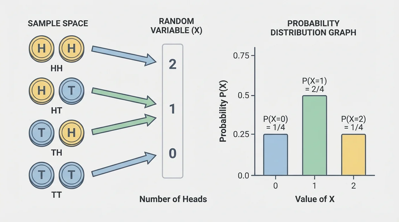
Suppose two coins are tossed. The sample space is \(\{HH, HT, TH, TT\}\). Let \(X\) represent the number of heads. Then \(X(HH)=2\), \(X(HT)=1\), \(X(TH)=1\), and \(X(TT)=0\). Notice that different outcomes can lead to the same random-variable value.
This is an important idea: the outcomes are not the same thing as the values of the random variable. The outcomes are \(HH\), \(HT\), \(TH\), and \(TT\). The values of \(X\) are \(0\), \(1\), and \(2\).
When a random variable can take only specific, countable values, it is called a discrete random variable. Most introductory probability distributions in high school are discrete. Examples include the number of goals scored in a game, the number of defective items in a box, or the amount of money won in a game.
If \(Y\) is the amount won by rolling a die and being paid according to the number of dots on the top face, then \(Y\) can be \(1,2,3,4,5,\) or \(6\). Those are countable values, so \(Y\) is discrete.
Not every quantity is discrete. If a random variable measures height, weight, or temperature, it can take many values in an interval, so it is usually considered continuous. This lesson focuses on discrete random variables because their probability distributions can be listed exactly.
To create a probability distribution, list each possible value of the random variable and find its probability. The probabilities must satisfy two conditions:
First, every probability is between \(0\) and \(1\), inclusive.
Second, the total probability must be \(1\):
\[\sum P(x)=1\]
For the two-coin example with \(X\) as the number of heads, the four outcomes are equally likely. Since each has probability \(\dfrac{1}{4}\), we combine outcomes that give the same value of \(X\):
| Value of \(X\) | Outcomes | Probability |
|---|---|---|
| \(0\) | \(TT\) | \(\dfrac{1}{4}\) |
| \(1\) | \(HT, TH\) | \(\dfrac{2}{4}=\dfrac{1}{2}\) |
| \(2\) | \(HH\) | \(\dfrac{1}{4}\) |
Table 1. Probability distribution for the number of heads in two coin tosses.
The probabilities add to \(\dfrac{1}{4}+\dfrac{1}{2}+\dfrac{1}{4}=1\), so this is a valid distribution.
When outcomes are equally likely, probability is found with \(\dfrac{\textrm{number of favorable outcomes}}{\textrm{total number of outcomes}}\). When several outcomes lead to the same random-variable value, add their probabilities.
[Figure 2] Sometimes the random variable is about money rather than counts. For example, let \(P\) be the profit from selling a concert ticket after paying fees. If different sales outcomes produce different profits, then each profit amount becomes a possible value of \(P\).
A probability distribution can be graphed using some of the same displays used for ordinary data distributions. For a discrete random variable, the most common graph is a bar graph. The horizontal axis shows the possible values of the random variable, and the vertical axis shows the probability of each value.
For the two-coin example, the bars are placed at \(x=0\), \(x=1\), and \(x=2\). Their heights are \(\dfrac{1}{4}\), \(\dfrac{1}{2}\), and \(\dfrac{1}{4}\).
This graph resembles a data bar graph, but there is an important difference. In a data distribution, the vertical axis may show frequency or relative frequency from actual observations. In a probability distribution, the vertical axis shows theoretical or assigned probabilities for the random variable.
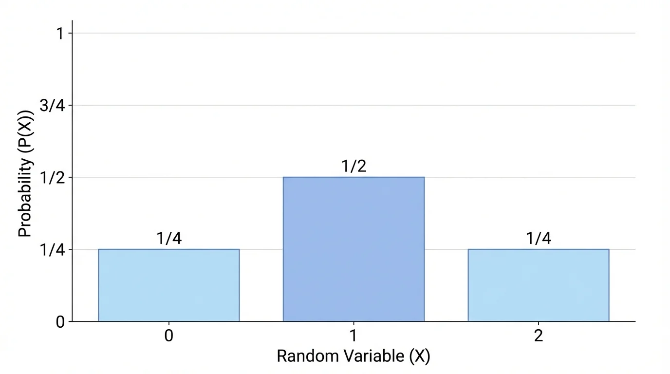
You can also use a table to display a probability distribution, and in some cases a dot plot can help highlight where the probabilities are concentrated. For instance, the value \(1\) in the two-coin example is more likely than \(0\) or \(2\), so the graph has its tallest bar at \(1\).
When reading such a graph, ask three questions: Which value is most likely? Which values are impossible? How spread out are the probabilities?
A spinner has four equal sections labeled \(1\), \(1\), \(2\), and \(5\). Let \(X\) be the number the spinner lands on. Build the probability distribution for \(X\).
Worked example
Step 1: List the possible values.
The spinner can land on \(1\), \(2\), or \(5\).
Step 2: Find each probability.
Because the sections are equal, each section has probability \(\dfrac{1}{4}\).
The value \(1\) appears on two sections, so \(P(X=1)=\dfrac{2}{4}=\dfrac{1}{2}\).
The value \(2\) appears on one section, so \(P(X=2)=\dfrac{1}{4}\).
The value \(5\) appears on one section, so \(P(X=5)=\dfrac{1}{4}\).
Step 3: Check the total probability.
\(\dfrac{1}{2}+\dfrac{1}{4}+\dfrac{1}{4}=1\)
The probability distribution is:
\[P(X=1)=\frac{1}{2}, \quad P(X=2)=\frac{1}{4}, \quad P(X=5)=\frac{1}{4}\]
If you graph this distribution, the bar above \(1\) is tallest, while the bars above \(2\) and \(5\) are shorter and equal in height.
A basketball player shoots two free throws. Assume each shot is made with probability \(0.8\), and the shots are independent. Let \(Y\) be the number of points scored, where each made shot is worth \(1\) point. Find the probability distribution of \(Y\).
Worked example
Step 1: List the possible values of the random variable.
The player can score \(0\), \(1\), or \(2\) points.
Step 2: Find the probability of \(0\) points.
This happens if both shots are missed.
\(P(Y=0)=0.2\cdot 0.2=0.04\)
Step 3: Find the probability of \(2\) points.
This happens if both shots are made.
\(P(Y=2)=0.8\cdot 0.8=0.64\)
Step 4: Find the probability of \(1\) point.
This happens in two ways: make the first and miss the second, or miss the first and make the second.
\(P(Y=1)=0.8\cdot 0.2+0.2\cdot 0.8=0.16+0.16=0.32\)
Step 5: Check the total.
\(0.04+0.32+0.64=1\)
The distribution is:
\[P(Y=0)=0.04, \quad P(Y=1)=0.32, \quad P(Y=2)=0.64\]
The probability distribution is heavily concentrated at \(2\), which matches intuition: a good free-throw shooter is most likely to make both shots.
A school store sells mystery snack bags for \(\$3\) each. The store owner estimates that the profit per bag, after costs, can be \(-1\), \(1\), or \(2\) dollars with probabilities \(0.1\), \(0.5\), and \(0.4\), respectively. Let \(Z\) be the profit in dollars per bag. Find the expected profit.
Worked example
Step 1: Write the expected value formula.
For a discrete random variable, the expected value is
\[E(Z)=\sum z\,P(Z=z)\]
Step 2: Multiply each value by its probability.
\((-1)(0.1)=-0.1\)
\((1)(0.5)=0.5\)
\((2)(0.4)=0.8\)
Step 3: Add the products.
\(E(Z)=-0.1+0.5+0.8=1.2\)
The expected profit is \(1.2\) dollars, so in the long run the store expects an average profit of \(\$1.20\) per bag.
The expected value does not have to be a value the random variable actually takes. Here, the profit is never exactly \(\$1.20\) on a single bag, but \(\$1.20\) is the long-run average over many sales.
An important use of a probability distribution is finding its expected value, which acts like a weighted average. Each possible value is weighted by how likely it is. This is why a graph can reveal not only what is possible but also what is typical over time when two choices have different shapes.
Expected value as a weighted average
If a discrete random variable \(X\) takes values \(x_1, x_2, x_3, ...\) with probabilities \(p_1, p_2, p_3, ...\), then
\[E(X)=x_1p_1+x_2p_2+x_3p_3+...\]
Values with larger probabilities influence the average more strongly than values with small probabilities.
[Figure 3] Suppose Game A pays \(2\) points with probability \(0.7\) and \(0\) points with probability \(0.3\). Game B pays \(6\) points with probability \(0.2\) and \(1\) point with probability \(0.8\). Their distributions look different: one is steadier, while the other has a rare larger reward.
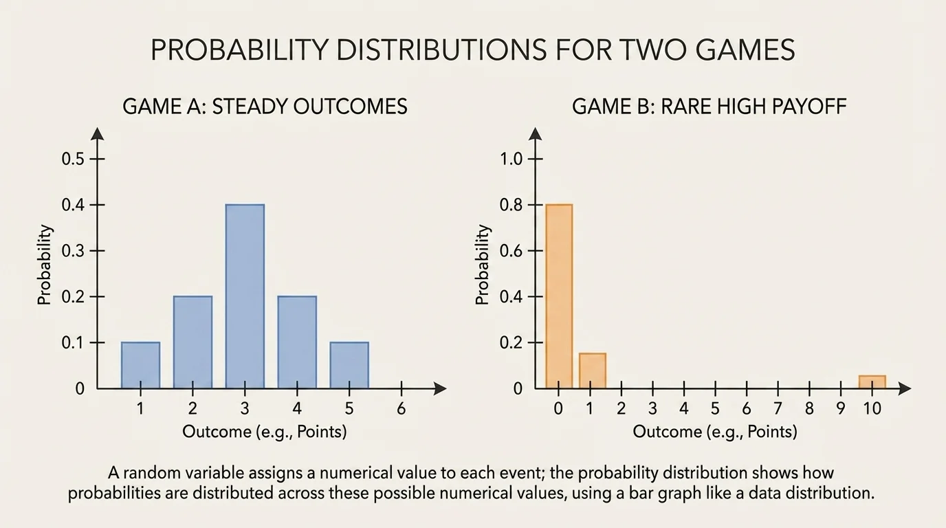
For Game A, \(E(A)=2(0.7)+0(0.3)=1.4\). For Game B, \(E(B)=6(0.2)+1(0.8)=1.2+0.8=2.0\). Based on expected value alone, Game B gives more points on average.
But expected value is not the whole story. Some people may prefer a steadier outcome even if the average is lower. That is why the graph shape matters. One distribution concentrates probability near a moderate score, while the other places more risk on a less likely high payoff.
A probability distribution graph can be described using many of the same ideas used for data distributions.
Center: The expected value gives a sense of the long-run balance point.
Spread: If probabilities are spread across many values, outcomes are less predictable.
Peaks: Tall bars show the most likely values.
Gaps: Missing bars show impossible values.
For example, in the two-coin distribution, there is no bar at \(x=3\) because getting three heads from two tosses is impossible. The symmetry visible in [Figure 2] also helps us see that \(0\) heads and \(2\) heads are equally likely.
Insurance companies do not predict exactly what will happen for one person. They rely on probability distributions and expected values over very large groups, which makes uncertain events more manageable.
Interpreting a distribution carefully also means distinguishing between a likely value and an average value. The value with the highest probability is called the mode, but the expected value may be somewhere else, especially if a large but rare outcome pulls the average.
One common mistake is mixing up the event and the random variable. An event might be "getting exactly one head," while the random variable value is simply \(1\).
Another mistake is forgetting to combine probabilities when different outcomes lead to the same value. In the two-coin example, both \(HT\) and \(TH\) contribute to \(X=1\).
A third mistake is making a graph that looks like a histogram. Histograms are used for grouped numerical data. For a discrete probability distribution, separate bars are usually better because the values are individual outcomes, not intervals.
It is also possible to define different random variables from the same sample space. If a die is rolled, one random variable might be the face value \(X\). Another might be \(W=1\) if the result is even and \(W=0\) if the result is odd. The experiment stays the same, but the numerical rule changes.
Random variables and probability distributions appear whenever people must make decisions under uncertainty.
In business, a manager may assign profits to different sales outcomes and compute expected profit before launching a product. In sports, analysts use distributions to estimate likely scores or the expected points from a strategy. In manufacturing, companies track the number of defective items in a sample. In medicine, researchers study probabilities of treatment success and side effects.
Even everyday choices involve these ideas. Choosing between two phone plans, two job offers, or two fundraising ideas often means comparing possible outcomes and their probabilities. A table or graph makes the comparison clearer, and expected value gives a useful summary.
| Context | Random Variable | Possible Values |
|---|---|---|
| Basketball | Points from two free throws | \(0,1,2\) |
| Business | Profit from one sale | \(-1,1,2\) |
| Quality control | Defective items in a sample | \(0,1,2,3,...\) |
| Games | Amount won | Depends on the rules |
Table 2. Examples of random variables in different real-world settings.
Whenever you can list the outcomes, assign a number to each one, and determine the probabilities, you can build a probability distribution. Once that distribution is graphed, you can see the pattern of uncertainty much more clearly than from words alone.